In [1]:

from __future__ import annotations

from functools import partial

import matplotlib.pyplot as plt
import numpy as np
import pandas as pd
import seaborn as sns
from numpy.polynomial.polynomial import Polynomial

from example_models.linear_chain import get_linear_chain_2v
from mxlpy import Model, Simulator, fns, npe, plot, scan, surrogates
from mxlpy.distributions import LogNormal, Normal, sample
from mxlpy.types import AbstractSurrogate, unwrap

from __future__ import annotations from functools import partial import matplotlib.pyplot as plt import numpy as np import pandas as pd import seaborn as sns from numpy.polynomial.polynomial import Polynomial from example_models.linear_chain import get_linear_chain_2v from mxlpy import Model, Simulator, fns, npe, plot, scan, surrogates from mxlpy.distributions import LogNormal, Normal, sample from mxlpy.types import AbstractSurrogate, unwrap

Mechanistic Learning¶

Mechanistic learning is the intersection of mechanistic modelling and machine learning.
mxlpy currently supports two such approaches: surrogates and neural posterior estimation.

In the following we will mostly use the mxlpy.surrogates and mxlpy.npe modules to learn about both approaches.

Surrogate models¶

Surrogate models replace whole parts of a mechanistic model (or even the entire model) with machine learning models.

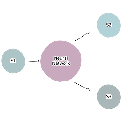
This allows combining together multiple models of arbitrary size, without having to worry about the internal state of each model.
They are especially useful for improving the description of boundary effects, e.g. a dynamic description of downstream consumption.

Manual construction¶

Surrogates can have return two kind of values in mxply: derived quantities and reactions.

We will start by defining a polynomial surrogate that will get the value of a variable x and output the derived quantity y.
Note that due to their nature surrogates can take multiple inputs and return multiple outputs, so we will always use iterables when defining them.

We then also add a derived value z that uses the output of our surrogate to see that we are getting the correct output.

In [2]:

m = Model()
m.add_variable("x", 1.0)
m.add_surrogate(
    "surrogate",
    surrogates.poly.Surrogate(
        model=Polynomial(coef=[2]),
        args=["x"],
        outputs=["y"],
    ),
)
m.add_derived("z", fns.add, args=["x", "y"])

# Check output
m.get_args()

m = Model() m.add_variable("x", 1.0) m.add_surrogate( "surrogate", surrogates.poly.Surrogate( model=Polynomial(coef=[2]), args=["x"], outputs=["y"], ), ) m.add_derived("z", fns.add, args=["x", "y"]) # Check output m.get_args()

Out[2]:

time    0.0
x       1.0
z       3.0
y       2.0
dtype: float64

Next we extend that idea to create a reaction.
The only thing we need to change here is to also add the stoichiometries of the respective output variable.

I've renamed the output to v1 here to fit convention, but that is not technically necessary.
mxlpy will always infer structurally into what kind of value your surrogate will be translated.

In [3]:

m = Model()
m.add_variable("x", 1.0)
m.add_surrogate(
    "surrogate",
    surrogates.poly.Surrogate(
        model=Polynomial(coef=[2]),
        args=["x"],
        outputs=["v1"],
        stoichiometries={"v1": {"x": -1}},
    ),
)
m.add_derived("z", fns.add, args=["x", "v1"])

# Check output
m.get_right_hand_side()

m = Model() m.add_variable("x", 1.0) m.add_surrogate( "surrogate", surrogates.poly.Surrogate( model=Polynomial(coef=[2]), args=["x"], outputs=["v1"], stoichiometries={"v1": {"x": -1}}, ), ) m.add_derived("z", fns.add, args=["x", "v1"]) # Check output m.get_right_hand_side()

Out[3]:

x   -2.0
dtype: float64

Note that if you have multiple outputs, it is perfectly fine for them to mix between derived values and reactions.

Surrogate(
    model=...,
    args=["x", "y"],
    outputs=["d1", "v1"],               # outputs derived value d1 and rate v1
    stoichiometries={"v1": {"x": -1}},  # only rate v1 is given stoichiometries
)

Training a surrogate from data and using it¶

We will start with a simple linear chain model

$$ \Large \varnothing \xrightarrow{v_1} x \xrightarrow{v_2} y \xrightarrow{v_3} \varnothing $$

where we want to read out the steady-state rate of $v_3$ dependent on the fixed concentration of $x$, while ignoring the inner state of the model.

$$ \Large x \xrightarrow{} ... \xrightarrow{v_3}$$

Since we need to fix a variable as an parameter, we can use the make_variable_static method to do that.

In [4]:

# Now "x" is a parameter
get_linear_chain_2v().make_variable_static("x").parameters

# Now "x" is a parameter get_linear_chain_2v().make_variable_static("x").parameters

Out[4]:

	value	unit
k1	1
k2	2
k3	1
x	1

And we can already create a function to create a model, which will take our surrogate as an input.

In [5]:

def get_model_with_surrogate(surrogate: AbstractSurrogate) -> Model:
    model = Model()
    model.add_variables({"x": 1.0, "z": 0.0})

    # Adding the surrogate
    model.add_surrogate(
        "surrogate",
        surrogate,
        args=["x"],
        outputs=["v2"],
        stoichiometries={
            "v2": {"x": -1, "z": 1},
        },
    )

    # Note that besides the surrogate we haven't defined any other reaction!
    # We could have though
    return model

def get_model_with_surrogate(surrogate: AbstractSurrogate) -> Model: model = Model() model.add_variables({"x": 1.0, "z": 0.0}) # Adding the surrogate model.add_surrogate( "surrogate", surrogate, args=["x"], outputs=["v2"], stoichiometries={ "v2": {"x": -1, "z": 1}, }, ) # Note that besides the surrogate we haven't defined any other reaction! # We could have though return model

Create data¶

The surrogates used in the following will all use the steady-state fluxes depending on the inputs.

We can thus create the necessary training data usign scan.steady_state.
Since this is usually a large amount of data, we recommend caching the results using Cache.

In [6]:

surrogate_features = pd.DataFrame({"x": np.geomspace(1e-12, 2.0, 21)})

surrogate_targets = scan.steady_state(
    get_linear_chain_2v().make_variable_static("x"),
    to_scan=surrogate_features,
).fluxes.loc[:, ["v3"]]

# It's always a good idea to check the inputs and outputs
fig, (ax1, ax2) = plot.two_axes(figsize=(6, 3), sharex=False)
_ = plot.violins(surrogate_features, ax=ax1)[1].set(
    title="Features", ylabel="Flux / a.u."
)
_ = plot.violins(surrogate_targets, ax=ax2)[1].set(
    title="Targets", ylabel="Flux / a.u."
)
plt.show()

surrogate_features = pd.DataFrame({"x": np.geomspace(1e-12, 2.0, 21)}) surrogate_targets = scan.steady_state( get_linear_chain_2v().make_variable_static("x"), to_scan=surrogate_features, ).fluxes.loc[:, ["v3"]] # It's always a good idea to check the inputs and outputs fig, (ax1, ax2) = plot.two_axes(figsize=(6, 3), sharex=False) _ = plot.violins(surrogate_features, ax=ax1)[1].set( title="Features", ylabel="Flux / a.u." ) _ = plot.violins(surrogate_targets, ax=ax2)[1].set( title="Targets", ylabel="Flux / a.u." ) plt.show()

  0%|          | 0/21 [00:00<?, ?it/s]

 43%|████▎     | 9/21 [00:00<00:00, 78.28it/s]

100%|██████████| 21/21 [00:00<00:00, 80.50it/s]

Polynomial surrogate¶

We can train our polynomial surrogate using train_polynomial_surrogate.
By default this will train polynomials for the degrees (1, 2, 3, 4, 5, 6, 7), but you can change that by using the degrees argument.
The function returns the trained surrogate and the training information for the different polynomial degrees.

Currently the polynomial surrogates are limited to a single feature and a single target

In [7]:

surrogate, info = surrogates.poly.train(
    surrogate_features["x"],
    surrogate_targets["v3"],
)

print("Model", surrogate.model, end="\n\n")
print(info["score"])

surrogate, info = surrogates.poly.train( surrogate_features["x"], surrogate_targets["v3"], ) print("Model", surrogate.model, end="\n\n") print(info["score"])

Model 2.0 + 2.0·(-1.0 + 1.0x)

degree
1     2.0
2     4.0
3     6.0
4     8.0
5    10.0
6    12.0
7    14.0
Name: score, dtype: float64

You can then insert the surrogate into the model using the function we defined earlier

In [8]:

concs, fluxes = unwrap(
    Simulator(get_model_with_surrogate(surrogate)).simulate(10).get_result()
)

fig, (ax1, ax2) = plot.two_axes(figsize=(8, 3))
plot.lines(concs, ax=ax1)
plot.lines(fluxes, ax=ax2)
ax1.set(xlabel="time / a.u.", ylabel="concentration / a.u.")
ax2.set(xlabel="time / a.u.", ylabel="flux / a.u.")
plt.show()

concs, fluxes = unwrap( Simulator(get_model_with_surrogate(surrogate)).simulate(10).get_result() ) fig, (ax1, ax2) = plot.two_axes(figsize=(8, 3)) plot.lines(concs, ax=ax1) plot.lines(fluxes, ax=ax2) ax1.set(xlabel="time / a.u.", ylabel="concentration / a.u.") ax2.set(xlabel="time / a.u.", ylabel="flux / a.u.") plt.show()

While polynomial regression can model nonlinear relationships between variables, it often struggles when the underlying relationship is more complex than a polynomial function.
You will learn about using neural networks in the next section.

Neural network surrogate using PyTorch¶

Neural networks are designed to capture highly complex and nonlinear relationships.
Through layers of neurons and activation functions, neural networks can learn intricate patterns that are not easily represented by e.g. a polynomial.
They have the flexibility to approximate any continuous function, given sufficient depth and appropriate training.

You can train a neural network surrogate based on the popular PyTorch library using train_torch_surrogate.
That function takes the features, targets and the number of epochs as inputs for it's training.

train_torch_surrogate returns the trained surrogate, as well as the training loss.
It is always a good idea to check whether that training loss approaches 0.

In [9]:

surrogate, loss = surrogates.torch.train(
    features=surrogate_features,
    targets=surrogate_targets,
    batch_size=100,
    epochs=250,
)

ax = loss.plot(ax=plt.subplots(figsize=(4, 2.5))[1])
ax.set_ylim(0, None)
plt.show()

surrogate, loss = surrogates.torch.train( features=surrogate_features, targets=surrogate_targets, batch_size=100, epochs=250, ) ax = loss.plot(ax=plt.subplots(figsize=(4, 2.5))[1]) ax.set_ylim(0, None) plt.show()

  0%|          | 0/250 [00:00<?, ?it/s]

 47%|████▋     | 117/250 [00:00<00:00, 1164.91it/s]

 94%|█████████▍| 236/250 [00:00<00:00, 1178.31it/s]

100%|██████████| 250/250 [00:00<00:00, 1172.24it/s]

As before, you can then insert the surrogate into the model using the function we defined earlier

In [10]:

concs, fluxes = unwrap(
    Simulator(get_model_with_surrogate(surrogate)).simulate(10).get_result()
)

fig, (ax1, ax2) = plot.two_axes(figsize=(8, 3))
plot.lines(concs, ax=ax1)
plot.lines(fluxes, ax=ax2)
ax1.set(xlabel="time / a.u.", ylabel="concentration / a.u.")
ax2.set(xlabel="time / a.u.", ylabel="flux / a.u.")
plt.show()

concs, fluxes = unwrap( Simulator(get_model_with_surrogate(surrogate)).simulate(10).get_result() ) fig, (ax1, ax2) = plot.two_axes(figsize=(8, 3)) plot.lines(concs, ax=ax1) plot.lines(fluxes, ax=ax2) ax1.set(xlabel="time / a.u.", ylabel="concentration / a.u.") ax2.set(xlabel="time / a.u.", ylabel="flux / a.u.") plt.show()

Re-entrant training¶

Quite often you don't know the amount of epochs you are going to need in order to reach the required loss.
In this case, you can directly use the TorchSurrogateTrainer class to continue training.

In [11]:

trainer = surrogates.torch.Trainer(
    features=surrogate_features,
    targets=surrogate_targets,
)

# First training epochs
trainer.train(epochs=100)
trainer.get_loss().plot(figsize=(4, 2.5)).set_ylim(0, None)
plt.show()

# Decide to continue training
trainer.train(epochs=150)
trainer.get_loss().plot(figsize=(4, 2.5)).set_ylim(0, None)
plt.show()

surrogate = trainer.get_surrogate(surrogate_outputs=["x"])

trainer = surrogates.torch.Trainer( features=surrogate_features, targets=surrogate_targets, ) # First training epochs trainer.train(epochs=100) trainer.get_loss().plot(figsize=(4, 2.5)).set_ylim(0, None) plt.show() # Decide to continue training trainer.train(epochs=150) trainer.get_loss().plot(figsize=(4, 2.5)).set_ylim(0, None) plt.show() surrogate = trainer.get_surrogate(surrogate_outputs=["x"])

  0%|          | 0/100 [00:00<?, ?it/s]

100%|██████████| 100/100 [00:00<00:00, 1187.13it/s]

  0%|          | 0/150 [00:00<?, ?it/s]

 79%|███████▊  | 118/150 [00:00<00:00, 1174.61it/s]

100%|██████████| 150/150 [00:00<00:00, 1167.94it/s]

Troubleshooting¶

It often can make sense to check specific predictions of the surrogate.
For example, what does it predict when the inputs are all 0?

In [12]:

print(surrogate.predict_raw(np.array([-0.1])))
print(surrogate.predict_raw(np.array([0.0])))
print(surrogate.predict_raw(np.array([0.1])))

print(surrogate.predict_raw(np.array([-0.1]))) print(surrogate.predict_raw(np.array([0.0]))) print(surrogate.predict_raw(np.array([0.1])))

[-0.01366527]
[-0.00174271]
[0.19745935]

Using keras instead of torch¶

If you installed keras, you can use it with exactly the same interface torch

In [13]:

surrogate, loss = surrogates.keras.train(
    features=surrogate_features,
    targets=surrogate_targets,
    batch_size=100,
    epochs=250,
)

ax = loss.plot(ax=plt.subplots(figsize=(4, 2.5))[1])
ax.set_ylim(0, None)
plt.show()

surrogate, loss = surrogates.keras.train( features=surrogate_features, targets=surrogate_targets, batch_size=100, epochs=250, ) ax = loss.plot(ax=plt.subplots(figsize=(4, 2.5))[1]) ax.set_ylim(0, None) plt.show()

2025-06-06 08:44:16.496240: E external/local_xla/xla/stream_executor/cuda/cuda_fft.cc:467] Unable to register cuFFT factory: Attempting to register factory for plugin cuFFT when one has already been registered
WARNING: All log messages before absl::InitializeLog() is called are written to STDERR
E0000 00:00:1749199456.510238    3316 cuda_dnn.cc:8579] Unable to register cuDNN factory: Attempting to register factory for plugin cuDNN when one has already been registered
E0000 00:00:1749199456.514503    3316 cuda_blas.cc:1407] Unable to register cuBLAS factory: Attempting to register factory for plugin cuBLAS when one has already been registered
W0000 00:00:1749199456.526154    3316 computation_placer.cc:177] computation placer already registered. Please check linkage and avoid linking the same target more than once.
W0000 00:00:1749199456.526165    3316 computation_placer.cc:177] computation placer already registered. Please check linkage and avoid linking the same target more than once.
W0000 00:00:1749199456.526167    3316 computation_placer.cc:177] computation placer already registered. Please check linkage and avoid linking the same target more than once.
W0000 00:00:1749199456.526168    3316 computation_placer.cc:177] computation placer already registered. Please check linkage and avoid linking the same target more than once.
2025-06-06 08:44:16.530402: I tensorflow/core/platform/cpu_feature_guard.cc:210] This TensorFlow binary is optimized to use available CPU instructions in performance-critical operations.
To enable the following instructions: AVX2 FMA, in other operations, rebuild TensorFlow with the appropriate compiler flags.

2025-06-06 08:44:21.353844: E external/local_xla/xla/stream_executor/cuda/cuda_platform.cc:51] failed call to cuInit: INTERNAL: CUDA error: Failed call to cuInit: UNKNOWN ERROR (303)

Neural posterior estimation¶

Neural posterior estimation answers the question: what parameters could have generated the data I measured?
Here you use an ODE model and prior knowledge about the parameters of interest to create synthetic data.
You then use the generated synthetic data as the features and the input parameters as the targets to train an inverse problem.
Once that training is successful, the neural network can now predict the input parameters for real world data.

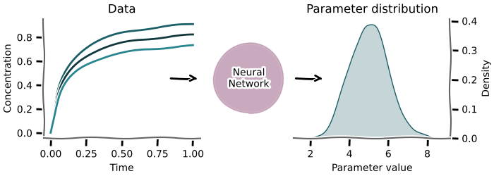
You can use this technique for both steady-state as well as time course data.
The only difference is in using scan.time_course.

Take care here to save the targets as well in case you use cached data :)

In [14]:

# Note that now the parameters are the targets
npe_targets = sample(
    {
        "k1": LogNormal(mean=1.0, sigma=0.3),
    },
    n=1_000,
)

# And the generated data are the features
npe_features = scan.steady_state(
    get_linear_chain_2v(),
    to_scan=npe_targets,
).results.loc[:, ["y", "v2", "v3"]]

# It's always a good idea to check the inputs and outputs
fig, (ax1, ax2) = plot.two_axes(figsize=(6, 3), sharex=False)
_ = plot.violins(npe_features, ax=ax1)[1].set(title="Features", ylabel="Flux / a.u.")
_ = plot.violins(npe_targets, ax=ax2)[1].set(title="Targets", ylabel="Flux / a.u.")
plt.show()

# Note that now the parameters are the targets npe_targets = sample( { "k1": LogNormal(mean=1.0, sigma=0.3), }, n=1_000, ) # And the generated data are the features npe_features = scan.steady_state( get_linear_chain_2v(), to_scan=npe_targets, ).results.loc[:, ["y", "v2", "v3"]] # It's always a good idea to check the inputs and outputs fig, (ax1, ax2) = plot.two_axes(figsize=(6, 3), sharex=False) _ = plot.violins(npe_features, ax=ax1)[1].set(title="Features", ylabel="Flux / a.u.") _ = plot.violins(npe_targets, ax=ax2)[1].set(title="Targets", ylabel="Flux / a.u.") plt.show()

  0%|          | 0/1000 [00:00<?, ?it/s]

  1%|          | 6/1000 [00:00<00:16, 59.97it/s]

  3%|▎         | 27/1000 [00:00<00:06, 142.79it/s]

  5%|▍         | 48/1000 [00:00<00:05, 170.45it/s]

  7%|▋         | 70/1000 [00:00<00:04, 187.38it/s]

  9%|▉         | 90/1000 [00:00<00:04, 190.56it/s]

 11%|█▏        | 114/1000 [00:00<00:04, 197.24it/s]

 14%|█▎        | 137/1000 [00:00<00:04, 203.69it/s]

 16%|█▌        | 158/1000 [00:00<00:04, 199.31it/s]

 18%|█▊        | 180/1000 [00:00<00:03, 205.23it/s]

 20%|██        | 201/1000 [00:01<00:03, 205.83it/s]

 22%|██▏       | 222/1000 [00:01<00:03, 201.83it/s]

 24%|██▍       | 245/1000 [00:01<00:03, 209.08it/s]

 27%|██▋       | 266/1000 [00:01<00:03, 204.49it/s]

 29%|██▊       | 287/1000 [00:01<00:03, 202.73it/s]

 31%|███       | 308/1000 [00:01<00:03, 200.05it/s]

 33%|███▎      | 331/1000 [00:01<00:03, 203.93it/s]

 35%|███▌      | 352/1000 [00:01<00:03, 205.20it/s]

 37%|███▋      | 374/1000 [00:01<00:03, 203.18it/s]

 40%|███▉      | 396/1000 [00:02<00:02, 204.69it/s]

 42%|████▏     | 417/1000 [00:02<00:02, 206.20it/s]

 44%|████▍     | 438/1000 [00:02<00:02, 205.45it/s]

 46%|████▌     | 459/1000 [00:02<00:02, 203.25it/s]

 48%|████▊     | 480/1000 [00:02<00:02, 196.30it/s]

 50%|█████     | 502/1000 [00:02<00:02, 202.11it/s]

 52%|█████▏    | 524/1000 [00:02<00:02, 203.40it/s]

 55%|█████▍    | 546/1000 [00:02<00:02, 207.26it/s]

 57%|█████▋    | 567/1000 [00:02<00:02, 205.54it/s]

 59%|█████▉    | 589/1000 [00:02<00:01, 208.38it/s]

 61%|██████    | 610/1000 [00:03<00:01, 204.27it/s]

 63%|██████▎   | 631/1000 [00:03<00:01, 205.93it/s]

 65%|██████▌   | 652/1000 [00:03<00:01, 204.64it/s]

 67%|██████▋   | 673/1000 [00:03<00:01, 205.64it/s]

 69%|██████▉   | 694/1000 [00:03<00:01, 202.12it/s]

 72%|███████▏  | 716/1000 [00:03<00:01, 202.81it/s]

 74%|███████▍  | 738/1000 [00:03<00:01, 203.87it/s]

 76%|███████▌  | 759/1000 [00:03<00:01, 204.66it/s]

 78%|███████▊  | 780/1000 [00:03<00:01, 204.77it/s]

 80%|████████  | 802/1000 [00:03<00:00, 204.57it/s]

 83%|████████▎ | 826/1000 [00:04<00:00, 205.12it/s]

 85%|████████▍ | 848/1000 [00:04<00:00, 208.95it/s]

 87%|████████▋ | 870/1000 [00:04<00:00, 205.78it/s]

 89%|████████▉ | 893/1000 [00:04<00:00, 211.91it/s]

 92%|█████████▏| 915/1000 [00:04<00:00, 209.09it/s]

 94%|█████████▎| 936/1000 [00:04<00:00, 206.72it/s]

 96%|█████████▌| 957/1000 [00:04<00:00, 205.66it/s]

 98%|█████████▊| 978/1000 [00:04<00:00, 205.28it/s]

100%|██████████| 1000/1000 [00:04<00:00, 207.15it/s]

100%|██████████| 1000/1000 [00:05<00:00, 198.83it/s]

Train NPE¶

You can then train your neural posterior estimator using npe.train_torch_ss_estimator (or npe.train_torch_time_course_estimator if you have time course data).

In [15]:

estimator, losses = npe.torch.train_steady_state(
    features=npe_features,
    targets=npe_targets,
    epochs=100,
    batch_size=100,
)

ax = losses.plot(figsize=(4, 2.5))
ax.set(xlabel="epoch", ylabel="loss")
ax.set_ylim(0, None)
plt.show()

estimator, losses = npe.torch.train_steady_state( features=npe_features, targets=npe_targets, epochs=100, batch_size=100, ) ax = losses.plot(figsize=(4, 2.5)) ax.set(xlabel="epoch", ylabel="loss") ax.set_ylim(0, None) plt.show()

  0%|          | 0/100 [00:00<?, ?it/s]

 10%|█         | 10/100 [00:00<00:00, 92.67it/s]

 20%|██        | 20/100 [00:00<00:00, 93.49it/s]

 30%|███       | 30/100 [00:00<00:00, 93.67it/s]

 40%|████      | 40/100 [00:00<00:00, 93.76it/s]

 50%|█████     | 50/100 [00:00<00:00, 93.87it/s]

 60%|██████    | 60/100 [00:00<00:00, 93.98it/s]

 70%|███████   | 70/100 [00:00<00:00, 94.01it/s]

 80%|████████  | 80/100 [00:00<00:00, 94.07it/s]

 90%|█████████ | 90/100 [00:00<00:00, 94.03it/s]

100%|██████████| 100/100 [00:01<00:00, 93.43it/s]

100%|██████████| 100/100 [00:01<00:00, 93.65it/s]

Sanity check: do prior and posterior match?¶

In [16]:

fig, (ax1, ax2) = plot.two_axes(figsize=(6, 2))

ax = sns.kdeplot(npe_targets, fill=True, ax=ax1)
ax.set_title("Prior")

posterior = estimator.predict(npe_features)
ax = sns.kdeplot(posterior, fill=True, ax=ax2)
ax.set_title("Posterior")
plt.show()

fig, (ax1, ax2) = plot.two_axes(figsize=(6, 2)) ax = sns.kdeplot(npe_targets, fill=True, ax=ax1) ax.set_title("Prior") posterior = estimator.predict(npe_features) ax = sns.kdeplot(posterior, fill=True, ax=ax2) ax.set_title("Posterior") plt.show()

Re-entrant training¶

As with the surrogates you often you don't know the amount of epochs you are going to need in order to reach the required loss.
For the neural posterior estimation you can use the npe.TorchSteadyStateTrainer and npe.TorchTimeCourseTrainer respectively to continue training.

In [17]:

trainer = npe.torch.SteadyStateTrainer(
    features=npe_features,
    targets=npe_targets,
)

# Initial training
trainer.train(epochs=20, batch_size=100)
trainer.get_loss().plot(figsize=(4, 2.5)).set_ylim(0, None)
plt.show()

# Continue training
trainer.train(epochs=20, batch_size=100)
trainer.get_loss().plot(figsize=(4, 2.5)).set_ylim(0, None)
plt.show()

# Get trainer if loss is deemed suitable
estimator = trainer.get_estimator()

trainer = npe.torch.SteadyStateTrainer( features=npe_features, targets=npe_targets, ) # Initial training trainer.train(epochs=20, batch_size=100) trainer.get_loss().plot(figsize=(4, 2.5)).set_ylim(0, None) plt.show() # Continue training trainer.train(epochs=20, batch_size=100) trainer.get_loss().plot(figsize=(4, 2.5)).set_ylim(0, None) plt.show() # Get trainer if loss is deemed suitable estimator = trainer.get_estimator()

  0%|          | 0/20 [00:00<?, ?it/s]

 50%|█████     | 10/20 [00:00<00:00, 92.34it/s]

100%|██████████| 20/20 [00:00<00:00, 92.65it/s]

100%|██████████| 20/20 [00:00<00:00, 92.36it/s]

  0%|          | 0/20 [00:00<?, ?it/s]

 50%|█████     | 10/20 [00:00<00:00, 93.62it/s]

100%|██████████| 20/20 [00:00<00:00, 93.24it/s]

100%|██████████| 20/20 [00:00<00:00, 93.01it/s]

First finish line

With that you now know most of what you will need from a day-to-day basis about labelled models in mxlpy.

Congratulations!

Custom loss function¶

You can use a custom loss function by simply injecting a function that takes the predicted tensor x and the data y and produces another tensor.

In [18]:

from typing import TYPE_CHECKING

import torch

from mxlpy import LinearLabelMapper, Simulator
from mxlpy.distributions import sample
from mxlpy.fns import michaelis_menten_1s
from mxlpy.parallel import parallelise

if TYPE_CHECKING:
    from mxlpy.types import AbstractEstimator

from typing import TYPE_CHECKING import torch from mxlpy import LinearLabelMapper, Simulator from mxlpy.distributions import sample from mxlpy.fns import michaelis_menten_1s from mxlpy.parallel import parallelise if TYPE_CHECKING: from mxlpy.types import AbstractEstimator

In [19]:

def mean_abs(x: torch.Tensor, y: torch.Tensor) -> torch.Tensor:
    return torch.mean(torch.abs(x - y))


trainer = surrogates.torch.Trainer(
    features=surrogate_features,
    targets=surrogate_targets,
    loss_fn=mean_abs,
)

trainer = npe.torch.SteadyStateTrainer(
    features=npe_features,
    targets=npe_targets,
    loss_fn=mean_abs,
)

trainer = npe.torch.TimeCourseTrainer(
    features=npe_features,
    targets=npe_targets,
    loss_fn=mean_abs,
)

def mean_abs(x: torch.Tensor, y: torch.Tensor) -> torch.Tensor: return torch.mean(torch.abs(x - y)) trainer = surrogates.torch.Trainer( features=surrogate_features, targets=surrogate_targets, loss_fn=mean_abs, ) trainer = npe.torch.SteadyStateTrainer( features=npe_features, targets=npe_targets, loss_fn=mean_abs, ) trainer = npe.torch.TimeCourseTrainer( features=npe_features, targets=npe_targets, loss_fn=mean_abs, )

Label NPE¶

In [20]:

# FIXME: todo
# Show how to change Adam settings or user other optimizers
# Show how to change the surrogate network

# FIXME: todo # Show how to change Adam settings or user other optimizers # Show how to change the surrogate network

In [21]:

def get_closed_cycle() -> tuple[Model, dict[str, int], dict[str, list[int]]]:
    """

    | Reaction       | Labelmap |
    | -------------- | -------- |
    | x1 ->[v1] x2   | [0, 1]   |
    | x2 ->[v2a] x3  | [0, 1]   |
    | x2 ->[v2b] x3  | [1, 0]   |
    | x3 ->[v3] x1   | [0, 1]   |

    """
    model = (
        Model()
        .add_parameters(
            {
                "vmax_1": 1.0,
                "km_1": 0.5,
                "vmax_2a": 1.0,
                "vmax_2b": 1.0,
                "km_2": 0.5,
                "vmax_3": 1.0,
                "km_3": 0.5,
            }
        )
        .add_variables({"x1": 1.0, "x2": 0.0, "x3": 0.0})
        .add_reaction(
            "v1",
            michaelis_menten_1s,
            stoichiometry={"x1": -1, "x2": 1},
            args=["x1", "vmax_1", "km_1"],
        )
        .add_reaction(
            "v2a",
            michaelis_menten_1s,
            stoichiometry={"x2": -1, "x3": 1},
            args=["x2", "vmax_2a", "km_2"],
        )
        .add_reaction(
            "v2b",
            michaelis_menten_1s,
            stoichiometry={"x2": -1, "x3": 1},
            args=["x2", "vmax_2b", "km_2"],
        )
        .add_reaction(
            "v3",
            michaelis_menten_1s,
            stoichiometry={"x3": -1, "x1": 1},
            args=["x3", "vmax_3", "km_3"],
        )
    )
    label_variables: dict[str, int] = {"x1": 2, "x2": 2, "x3": 2}
    label_maps: dict[str, list[int]] = {
        "v1": [0, 1],
        "v2a": [0, 1],
        "v2b": [1, 0],
        "v3": [0, 1],
    }
    return model, label_variables, label_maps

def get_closed_cycle() -> tuple[Model, dict[str, int], dict[str, list[int]]]: """ | Reaction | Labelmap | | -------------- | -------- | | x1 ->[v1] x2 | [0, 1] | | x2 ->[v2a] x3 | [0, 1] | | x2 ->[v2b] x3 | [1, 0] | | x3 ->[v3] x1 | [0, 1] | """ model = ( Model() .add_parameters( { "vmax_1": 1.0, "km_1": 0.5, "vmax_2a": 1.0, "vmax_2b": 1.0, "km_2": 0.5, "vmax_3": 1.0, "km_3": 0.5, } ) .add_variables({"x1": 1.0, "x2": 0.0, "x3": 0.0}) .add_reaction( "v1", michaelis_menten_1s, stoichiometry={"x1": -1, "x2": 1}, args=["x1", "vmax_1", "km_1"], ) .add_reaction( "v2a", michaelis_menten_1s, stoichiometry={"x2": -1, "x3": 1}, args=["x2", "vmax_2a", "km_2"], ) .add_reaction( "v2b", michaelis_menten_1s, stoichiometry={"x2": -1, "x3": 1}, args=["x2", "vmax_2b", "km_2"], ) .add_reaction( "v3", michaelis_menten_1s, stoichiometry={"x3": -1, "x1": 1}, args=["x3", "vmax_3", "km_3"], ) ) label_variables: dict[str, int] = {"x1": 2, "x2": 2, "x3": 2} label_maps: dict[str, list[int]] = { "v1": [0, 1], "v2a": [0, 1], "v2b": [1, 0], "v3": [0, 1], } return model, label_variables, label_maps

In [22]:

def _worker(
    x: tuple[tuple[int, pd.Series], tuple[int, pd.Series]],
    mapper: LinearLabelMapper,
    time: float,
    initial_labels: dict[str, int | list[int]],
) -> pd.Series:
    (_, y_ss), (_, v_ss) = x
    return unwrap(
        Simulator(mapper.build_model(y_ss, v_ss, initial_labels=initial_labels))
        .simulate(time)
        .get_result()
    ).variables.iloc[-1]


def get_label_distribution_at_time(
    model: Model,
    label_variables: dict[str, int],
    label_maps: dict[str, list[int]],
    time: float,
    initial_labels: dict[str, int | list[int]],
    ss_concs: pd.DataFrame,
    ss_fluxes: pd.DataFrame,
) -> pd.DataFrame:
    mapper = LinearLabelMapper(
        model,
        label_variables=label_variables,
        label_maps=label_maps,
    )

    return pd.DataFrame(
        dict(
            parallelise(
                partial(
                    _worker, mapper=mapper, time=time, initial_labels=initial_labels
                ),
                inputs=list(
                    enumerate(
                        zip(
                            ss_concs.iterrows(),
                            ss_fluxes.iterrows(),
                            strict=True,
                        )
                    )
                ),  # type: ignore
                cache=None,
            )
        ),
        dtype=float,
    ).T


def inverse_parameter_elasticity(
    estimator: AbstractEstimator,
    datum: pd.Series,
    *,
    normalized: bool = True,
    displacement: float = 1e-4,
) -> pd.DataFrame:
    ref = estimator.predict(datum).iloc[0, :]

    coefs = {}
    for name, value in datum.items():
        up = coefs[name] = estimator.predict(
            pd.Series(datum.to_dict() | {name: value * 1 + displacement})
        ).iloc[0, :]
        down = coefs[name] = estimator.predict(
            pd.Series(datum.to_dict() | {name: value * 1 - displacement})
        ).iloc[0, :]
        coefs[name] = (up - down) / (2 * displacement * value)

    coefs = pd.DataFrame(coefs)
    if normalized:
        coefs *= datum / ref.to_numpy()

    return coefs

def _worker( x: tuple[tuple[int, pd.Series], tuple[int, pd.Series]], mapper: LinearLabelMapper, time: float, initial_labels: dict[str, int | list[int]], ) -> pd.Series: (_, y_ss), (_, v_ss) = x return unwrap( Simulator(mapper.build_model(y_ss, v_ss, initial_labels=initial_labels)) .simulate(time) .get_result() ).variables.iloc[-1] def get_label_distribution_at_time( model: Model, label_variables: dict[str, int], label_maps: dict[str, list[int]], time: float, initial_labels: dict[str, int | list[int]], ss_concs: pd.DataFrame, ss_fluxes: pd.DataFrame, ) -> pd.DataFrame: mapper = LinearLabelMapper( model, label_variables=label_variables, label_maps=label_maps, ) return pd.DataFrame( dict( parallelise( partial( _worker, mapper=mapper, time=time, initial_labels=initial_labels ), inputs=list( enumerate( zip( ss_concs.iterrows(), ss_fluxes.iterrows(), strict=True, ) ) ), # type: ignore cache=None, ) ), dtype=float, ).T def inverse_parameter_elasticity( estimator: AbstractEstimator, datum: pd.Series, *, normalized: bool = True, displacement: float = 1e-4, ) -> pd.DataFrame: ref = estimator.predict(datum).iloc[0, :] coefs = {} for name, value in datum.items(): up = coefs[name] = estimator.predict( pd.Series(datum.to_dict() | {name: value * 1 + displacement}) ).iloc[0, :] down = coefs[name] = estimator.predict( pd.Series(datum.to_dict() | {name: value * 1 - displacement}) ).iloc[0, :] coefs[name] = (up - down) / (2 * displacement * value) coefs = pd.DataFrame(coefs) if normalized: coefs *= datum / ref.to_numpy() return coefs

In [23]:

model, label_variables, label_maps = get_closed_cycle()

ss_concs, ss_fluxes = unwrap(
    Simulator(model)
    .update_parameters({"vmax_2a": 1.0, "vmax_2b": 0.5})
    .simulate_to_steady_state()
    .get_result()
)
mapper = LinearLabelMapper(
    model,
    label_variables=label_variables,
    label_maps=label_maps,
)

_, axs = plot.relative_label_distribution(
    mapper,
    unwrap(
        Simulator(
            mapper.build_model(
                ss_concs.iloc[-1], ss_fluxes.iloc[-1], initial_labels={"x1": 0}
            )
        )
        .simulate(5)
        .get_result()
    ).variables,
    sharey=True,
    n_cols=3,
)

axs[0, 0].set_ylabel("Relative label distribution")
axs[0, 1].set_xlabel("Time / s")
plt.show()

model, label_variables, label_maps = get_closed_cycle() ss_concs, ss_fluxes = unwrap( Simulator(model) .update_parameters({"vmax_2a": 1.0, "vmax_2b": 0.5}) .simulate_to_steady_state() .get_result() ) mapper = LinearLabelMapper( model, label_variables=label_variables, label_maps=label_maps, ) _, axs = plot.relative_label_distribution( mapper, unwrap( Simulator( mapper.build_model( ss_concs.iloc[-1], ss_fluxes.iloc[-1], initial_labels={"x1": 0} ) ) .simulate(5) .get_result() ).variables, sharey=True, n_cols=3, ) axs[0, 0].set_ylabel("Relative label distribution") axs[0, 1].set_xlabel("Time / s") plt.show()

In [24]:

surrogate_targets = sample(
    {
        "vmax_2b": Normal(0.5, 0.1),
    },
    n=1000,
).clip(lower=0)

ax = sns.kdeplot(surrogate_targets, fill=True)
ax.set_title("Prior")

surrogate_targets = sample( { "vmax_2b": Normal(0.5, 0.1), }, n=1000, ).clip(lower=0) ax = sns.kdeplot(surrogate_targets, fill=True) ax.set_title("Prior")

Out[24]:

Text(0.5, 1.0, 'Prior')

In [25]:

ss_concs, ss_fluxes = scan.steady_state(
    model,
    to_scan=surrogate_targets,
)

ss_concs, ss_fluxes = scan.steady_state( model, to_scan=surrogate_targets, )

  0%|          | 0/1000 [00:00<?, ?it/s]

  0%|          | 1/1000 [00:00<09:04,  1.83it/s]

  1%|          | 11/1000 [00:00<00:45, 21.71it/s]

  2%|▏         | 23/1000 [00:00<00:22, 42.77it/s]

  4%|▎         | 35/1000 [00:00<00:16, 59.39it/s]

  5%|▍         | 47/1000 [00:00<00:13, 72.45it/s]

  6%|▌         | 59/1000 [00:01<00:11, 82.23it/s]

  7%|▋         | 71/1000 [00:01<00:10, 89.24it/s]

  8%|▊         | 83/1000 [00:01<00:09, 94.63it/s]

 10%|▉         | 95/1000 [00:01<00:09, 98.12it/s]

 11%|█         | 107/1000 [00:01<00:08, 100.73it/s]

 12%|█▏        | 119/1000 [00:01<00:08, 102.57it/s]

 13%|█▎        | 131/1000 [00:01<00:08, 103.95it/s]

 14%|█▍        | 143/1000 [00:01<00:08, 104.90it/s]

 16%|█▌        | 155/1000 [00:01<00:07, 105.92it/s]

 17%|█▋        | 167/1000 [00:02<00:07, 106.20it/s]

 18%|█▊        | 179/1000 [00:02<00:07, 106.78it/s]

 19%|█▉        | 190/1000 [00:02<00:07, 107.66it/s]

 20%|██        | 201/1000 [00:02<00:07, 105.84it/s]

 21%|██        | 212/1000 [00:02<00:07, 105.57it/s]

 22%|██▏       | 224/1000 [00:02<00:07, 106.00it/s]

 24%|██▎       | 236/1000 [00:02<00:07, 106.28it/s]

 25%|██▍       | 248/1000 [00:02<00:07, 106.55it/s]

 26%|██▌       | 260/1000 [00:02<00:06, 106.85it/s]

 27%|██▋       | 271/1000 [00:03<00:06, 105.91it/s]

 28%|██▊       | 282/1000 [00:03<00:06, 103.54it/s]

 29%|██▉       | 293/1000 [00:03<00:07, 98.62it/s] 

 30%|███       | 304/1000 [00:03<00:06, 100.18it/s]

 32%|███▏      | 316/1000 [00:03<00:06, 100.93it/s]

 33%|███▎      | 328/1000 [00:03<00:06, 102.77it/s]

 34%|███▍      | 340/1000 [00:03<00:06, 104.30it/s]

 35%|███▌      | 352/1000 [00:03<00:06, 105.44it/s]

 36%|███▋      | 364/1000 [00:03<00:06, 105.80it/s]

 38%|███▊      | 376/1000 [00:04<00:05, 107.08it/s]

 39%|███▉      | 388/1000 [00:04<00:05, 107.31it/s]

 40%|████      | 400/1000 [00:04<00:05, 106.97it/s]

 41%|████      | 412/1000 [00:04<00:05, 107.10it/s]

 42%|████▏     | 424/1000 [00:04<00:05, 107.04it/s]

 44%|████▎     | 435/1000 [00:04<00:05, 107.66it/s]

 45%|████▍     | 447/1000 [00:04<00:05, 107.61it/s]

 46%|████▌     | 458/1000 [00:04<00:05, 106.92it/s]

 47%|████▋     | 469/1000 [00:04<00:05, 106.04it/s]

 48%|████▊     | 480/1000 [00:05<00:04, 107.15it/s]

 49%|████▉     | 492/1000 [00:05<00:04, 106.93it/s]

 50%|█████     | 504/1000 [00:05<00:04, 108.18it/s]

 52%|█████▏    | 515/1000 [00:05<00:04, 102.96it/s]

 53%|█████▎    | 526/1000 [00:05<00:04, 102.17it/s]

 54%|█████▎    | 537/1000 [00:05<00:04, 103.92it/s]

 55%|█████▍    | 548/1000 [00:05<00:04, 102.25it/s]

 56%|█████▌    | 560/1000 [00:05<00:04, 104.07it/s]

 57%|█████▋    | 572/1000 [00:05<00:04, 105.33it/s]

 58%|█████▊    | 584/1000 [00:06<00:03, 106.08it/s]

 60%|█████▉    | 596/1000 [00:06<00:03, 106.31it/s]

 61%|██████    | 608/1000 [00:06<00:03, 106.94it/s]

 62%|██████▏   | 620/1000 [00:06<00:03, 107.34it/s]

 63%|██████▎   | 631/1000 [00:06<00:03, 107.00it/s]

 64%|██████▍   | 642/1000 [00:06<00:03, 105.26it/s]

 65%|██████▌   | 653/1000 [00:06<00:03, 106.19it/s]

 66%|██████▋   | 664/1000 [00:06<00:03, 106.66it/s]

 68%|██████▊   | 675/1000 [00:06<00:03, 105.19it/s]

 69%|██████▊   | 686/1000 [00:07<00:02, 105.82it/s]

 70%|██████▉   | 698/1000 [00:07<00:02, 105.81it/s]

 71%|███████   | 710/1000 [00:07<00:02, 106.13it/s]

 72%|███████▏  | 722/1000 [00:07<00:02, 106.62it/s]

 73%|███████▎  | 734/1000 [00:07<00:02, 106.78it/s]

 75%|███████▍  | 746/1000 [00:07<00:02, 106.86it/s]

 76%|███████▌  | 758/1000 [00:07<00:02, 106.54it/s]

 77%|███████▋  | 770/1000 [00:07<00:02, 107.27it/s]

 78%|███████▊  | 782/1000 [00:07<00:02, 107.41it/s]

 79%|███████▉  | 794/1000 [00:08<00:01, 106.54it/s]

 81%|████████  | 806/1000 [00:08<00:01, 106.82it/s]

 82%|████████▏ | 818/1000 [00:08<00:01, 106.80it/s]

 83%|████████▎ | 830/1000 [00:08<00:01, 106.97it/s]

 84%|████████▍ | 841/1000 [00:08<00:01, 107.57it/s]

 85%|████████▌ | 852/1000 [00:08<00:01, 107.25it/s]

 86%|████████▋ | 863/1000 [00:08<00:01, 106.84it/s]

 87%|████████▋ | 874/1000 [00:08<00:01, 106.29it/s]

 88%|████████▊ | 885/1000 [00:08<00:01, 105.46it/s]

 90%|████████▉ | 897/1000 [00:09<00:00, 105.12it/s]

 91%|█████████ | 909/1000 [00:09<00:00, 105.31it/s]

 92%|█████████▏| 921/1000 [00:09<00:00, 106.17it/s]

 93%|█████████▎| 933/1000 [00:09<00:00, 106.74it/s]

 94%|█████████▍| 945/1000 [00:09<00:00, 106.93it/s]

 96%|█████████▌| 957/1000 [00:09<00:00, 106.93it/s]

 97%|█████████▋| 969/1000 [00:09<00:00, 106.91it/s]

 98%|█████████▊| 981/1000 [00:09<00:00, 107.16it/s]

 99%|█████████▉| 993/1000 [00:09<00:00, 107.49it/s]

100%|██████████| 1000/1000 [00:10<00:00, 99.62it/s]

In [26]:

fig, (ax1, ax2) = plt.subplots(1, 2, figsize=(12, 4))
_, ax = plot.violins(ss_concs, ax=ax1)
ax.set_ylabel("Concentration / a.u.")
_, ax = plot.violins(ss_fluxes, ax=ax2)
ax.set_ylabel("Flux / a.u.")

fig, (ax1, ax2) = plt.subplots(1, 2, figsize=(12, 4)) _, ax = plot.violins(ss_concs, ax=ax1) ax.set_ylabel("Concentration / a.u.") _, ax = plot.violins(ss_fluxes, ax=ax2) ax.set_ylabel("Flux / a.u.")

Out[26]:

Text(0, 0.5, 'Flux / a.u.')

In [27]:

surrogate_features = get_label_distribution_at_time(
    model=model,
    label_variables=label_variables,
    label_maps=label_maps,
    time=5,
    ss_concs=ss_concs,
    ss_fluxes=ss_fluxes,
    initial_labels={"x1": 0},
)
_, ax = plot.violins(surrogate_features)
ax.set_ylabel("Relative label distribution")

surrogate_features = get_label_distribution_at_time( model=model, label_variables=label_variables, label_maps=label_maps, time=5, ss_concs=ss_concs, ss_fluxes=ss_fluxes, initial_labels={"x1": 0}, ) _, ax = plot.violins(surrogate_features) ax.set_ylabel("Relative label distribution")

  0%|          | 0/1000 [00:00<?, ?it/s]

  0%|          | 1/1000 [00:00<02:09,  7.71it/s]

  1%|          | 9/1000 [00:00<00:23, 41.44it/s]

  2%|▏         | 17/1000 [00:00<00:18, 53.94it/s]

  2%|▎         | 25/1000 [00:00<00:16, 60.07it/s]

  3%|▎         | 33/1000 [00:00<00:15, 63.31it/s]

  4%|▍         | 41/1000 [00:00<00:14, 64.87it/s]

  5%|▍         | 49/1000 [00:00<00:14, 65.92it/s]

  6%|▌         | 57/1000 [00:00<00:14, 66.76it/s]

  6%|▋         | 65/1000 [00:01<00:13, 67.15it/s]

  7%|▋         | 73/1000 [00:01<00:13, 66.84it/s]

  8%|▊         | 81/1000 [00:01<00:13, 66.67it/s]

  9%|▉         | 89/1000 [00:01<00:13, 67.08it/s]

 10%|▉         | 97/1000 [00:01<00:13, 66.85it/s]

 10%|█         | 105/1000 [00:01<00:13, 67.84it/s]

 11%|█▏        | 113/1000 [00:01<00:13, 68.02it/s]

 12%|█▏        | 121/1000 [00:01<00:12, 68.25it/s]

 13%|█▎        | 129/1000 [00:02<00:12, 68.42it/s]

 14%|█▎        | 137/1000 [00:02<00:12, 69.30it/s]

 14%|█▍        | 145/1000 [00:02<00:12, 69.33it/s]

 15%|█▌        | 153/1000 [00:02<00:12, 68.79it/s]

 16%|█▌        | 161/1000 [00:02<00:12, 68.84it/s]

 17%|█▋        | 169/1000 [00:02<00:12, 69.09it/s]

 18%|█▊        | 177/1000 [00:02<00:12, 68.31it/s]

 18%|█▊        | 185/1000 [00:02<00:11, 68.38it/s]

 19%|█▉        | 193/1000 [00:02<00:11, 68.16it/s]

 20%|██        | 201/1000 [00:03<00:11, 68.83it/s]

 21%|██        | 209/1000 [00:03<00:11, 68.12it/s]

 22%|██▏       | 217/1000 [00:03<00:11, 67.34it/s]

 22%|██▎       | 225/1000 [00:03<00:11, 67.95it/s]

 23%|██▎       | 233/1000 [00:03<00:11, 68.24it/s]

 24%|██▍       | 240/1000 [00:03<00:11, 68.14it/s]

 25%|██▍       | 247/1000 [00:03<00:11, 66.58it/s]

 25%|██▌       | 254/1000 [00:03<00:11, 66.54it/s]

 26%|██▌       | 261/1000 [00:03<00:10, 67.21it/s]

 27%|██▋       | 268/1000 [00:04<00:10, 67.09it/s]

 28%|██▊       | 275/1000 [00:04<00:11, 65.89it/s]

 28%|██▊       | 282/1000 [00:04<00:10, 66.77it/s]

 29%|██▉       | 290/1000 [00:04<00:10, 66.40it/s]

 30%|██▉       | 298/1000 [00:04<00:10, 67.12it/s]

 31%|███       | 306/1000 [00:04<00:10, 68.28it/s]

 31%|███▏      | 314/1000 [00:04<00:10, 67.96it/s]

 32%|███▏      | 322/1000 [00:04<00:10, 67.42it/s]

 33%|███▎      | 330/1000 [00:04<00:09, 67.89it/s]

 34%|███▍      | 338/1000 [00:05<00:09, 67.34it/s]

 35%|███▍      | 346/1000 [00:05<00:09, 67.29it/s]

 35%|███▌      | 354/1000 [00:05<00:09, 67.59it/s]

 36%|███▌      | 362/1000 [00:05<00:09, 67.74it/s]

 37%|███▋      | 370/1000 [00:05<00:09, 68.63it/s]

 38%|███▊      | 377/1000 [00:05<00:09, 68.55it/s]

 38%|███▊      | 384/1000 [00:05<00:08, 68.72it/s]

 39%|███▉      | 392/1000 [00:05<00:08, 67.94it/s]

 40%|████      | 400/1000 [00:06<00:08, 67.82it/s]

 41%|████      | 408/1000 [00:06<00:08, 67.88it/s]

 42%|████▏     | 415/1000 [00:06<00:08, 67.64it/s]

 42%|████▏     | 422/1000 [00:06<00:08, 66.68it/s]

 43%|████▎     | 429/1000 [00:06<00:08, 66.71it/s]

 44%|████▎     | 437/1000 [00:06<00:08, 66.78it/s]

 44%|████▍     | 444/1000 [00:06<00:08, 67.21it/s]

 45%|████▌     | 451/1000 [00:06<00:08, 67.32it/s]

 46%|████▌     | 458/1000 [00:06<00:07, 67.96it/s]

 46%|████▋     | 465/1000 [00:06<00:08, 64.67it/s]

 47%|████▋     | 473/1000 [00:07<00:08, 65.86it/s]

 48%|████▊     | 480/1000 [00:07<00:07, 66.66it/s]

 49%|████▉     | 488/1000 [00:07<00:07, 66.61it/s]

 50%|████▉     | 496/1000 [00:07<00:07, 67.59it/s]

 50%|█████     | 503/1000 [00:07<00:07, 67.73it/s]

 51%|█████     | 510/1000 [00:07<00:07, 66.35it/s]

 52%|█████▏    | 517/1000 [00:07<00:07, 64.93it/s]

 52%|█████▎    | 525/1000 [00:07<00:07, 66.64it/s]

 53%|█████▎    | 533/1000 [00:07<00:06, 66.96it/s]

 54%|█████▍    | 541/1000 [00:08<00:06, 67.23it/s]

 55%|█████▍    | 549/1000 [00:08<00:06, 66.27it/s]

 56%|█████▌    | 557/1000 [00:08<00:06, 66.91it/s]

 56%|█████▋    | 565/1000 [00:08<00:06, 66.84it/s]

 57%|█████▋    | 573/1000 [00:08<00:06, 67.45it/s]

 58%|█████▊    | 581/1000 [00:08<00:06, 67.82it/s]

 59%|█████▉    | 589/1000 [00:08<00:06, 67.61it/s]

 60%|█████▉    | 597/1000 [00:08<00:05, 67.63it/s]

 60%|██████    | 605/1000 [00:09<00:05, 67.91it/s]

 61%|██████▏   | 613/1000 [00:09<00:05, 67.54it/s]

 62%|██████▏   | 621/1000 [00:09<00:05, 66.67it/s]

 63%|██████▎   | 629/1000 [00:09<00:05, 67.65it/s]

 64%|██████▎   | 637/1000 [00:09<00:05, 68.48it/s]

 64%|██████▍   | 645/1000 [00:09<00:05, 69.05it/s]

 65%|██████▌   | 652/1000 [00:09<00:05, 69.05it/s]

 66%|██████▌   | 660/1000 [00:09<00:04, 68.47it/s]

 67%|██████▋   | 668/1000 [00:09<00:04, 67.42it/s]

 68%|██████▊   | 676/1000 [00:10<00:04, 68.21it/s]

 68%|██████▊   | 684/1000 [00:10<00:04, 67.34it/s]

 69%|██████▉   | 692/1000 [00:10<00:04, 67.86it/s]

 70%|███████   | 700/1000 [00:10<00:04, 66.67it/s]

 71%|███████   | 708/1000 [00:10<00:04, 67.34it/s]

 72%|███████▏  | 716/1000 [00:10<00:04, 68.27it/s]

 72%|███████▏  | 724/1000 [00:10<00:04, 67.93it/s]

 73%|███████▎  | 732/1000 [00:10<00:03, 67.87it/s]

 74%|███████▍  | 740/1000 [00:11<00:03, 67.41it/s]

 75%|███████▍  | 748/1000 [00:11<00:03, 67.47it/s]

 76%|███████▌  | 755/1000 [00:11<00:03, 67.77it/s]

 76%|███████▌  | 762/1000 [00:11<00:03, 66.10it/s]

 77%|███████▋  | 769/1000 [00:11<00:03, 65.61it/s]

 78%|███████▊  | 777/1000 [00:11<00:03, 66.89it/s]

 78%|███████▊  | 784/1000 [00:11<00:03, 66.65it/s]

 79%|███████▉  | 792/1000 [00:11<00:03, 67.02it/s]

 80%|████████  | 800/1000 [00:11<00:02, 67.44it/s]

 81%|████████  | 807/1000 [00:12<00:02, 67.73it/s]

 81%|████████▏ | 814/1000 [00:12<00:02, 66.10it/s]

 82%|████████▏ | 821/1000 [00:12<00:02, 66.84it/s]

 83%|████████▎ | 828/1000 [00:12<00:02, 66.89it/s]

 84%|████████▎ | 835/1000 [00:12<00:02, 65.99it/s]

 84%|████████▍ | 842/1000 [00:12<00:02, 66.93it/s]

 85%|████████▌ | 850/1000 [00:12<00:02, 66.97it/s]

 86%|████████▌ | 858/1000 [00:12<00:02, 66.65it/s]

 87%|████████▋ | 866/1000 [00:12<00:01, 67.35it/s]

 87%|████████▋ | 874/1000 [00:13<00:01, 67.91it/s]

 88%|████████▊ | 882/1000 [00:13<00:01, 66.67it/s]

 89%|████████▉ | 890/1000 [00:13<00:01, 66.47it/s]

 90%|████████▉ | 898/1000 [00:13<00:01, 66.94it/s]

 91%|█████████ | 906/1000 [00:13<00:01, 67.12it/s]

 91%|█████████▏| 914/1000 [00:13<00:01, 67.59it/s]

 92%|█████████▏| 922/1000 [00:13<00:01, 67.34it/s]

 93%|█████████▎| 930/1000 [00:13<00:01, 69.03it/s]

 94%|█████████▎| 937/1000 [00:13<00:00, 69.13it/s]

 94%|█████████▍| 944/1000 [00:14<00:00, 69.29it/s]

 95%|█████████▌| 952/1000 [00:14<00:00, 68.12it/s]

 96%|█████████▌| 960/1000 [00:14<00:00, 67.52it/s]

 97%|█████████▋| 968/1000 [00:14<00:00, 67.31it/s]

 98%|█████████▊| 976/1000 [00:14<00:00, 67.24it/s]

 98%|█████████▊| 984/1000 [00:14<00:00, 67.38it/s]

 99%|█████████▉| 992/1000 [00:14<00:00, 67.35it/s]

100%|██████████| 1000/1000 [00:14<00:00, 70.18it/s]

100%|██████████| 1000/1000 [00:15<00:00, 66.42it/s]

Out[27]:

Text(0, 0.5, 'Relative label distribution')

In [28]:

estimator, losses = npe.torch.train_steady_state(
    features=surrogate_features,
    targets=surrogate_targets,
    batch_size=100,
    epochs=250,
)

ax = losses.plot()
ax.set_ylim(0, None)

estimator, losses = npe.torch.train_steady_state( features=surrogate_features, targets=surrogate_targets, batch_size=100, epochs=250, ) ax = losses.plot() ax.set_ylim(0, None)

  0%|          | 0/250 [00:00<?, ?it/s]

  4%|▎         | 9/250 [00:00<00:02, 88.80it/s]

  8%|▊         | 19/250 [00:00<00:02, 91.28it/s]

 12%|█▏        | 29/250 [00:00<00:02, 92.02it/s]

 16%|█▌        | 39/250 [00:00<00:02, 92.49it/s]

 20%|█▉        | 49/250 [00:00<00:02, 92.56it/s]

 24%|██▎       | 59/250 [00:00<00:02, 92.54it/s]

 28%|██▊       | 69/250 [00:00<00:01, 92.57it/s]

 32%|███▏      | 79/250 [00:00<00:01, 92.47it/s]

 36%|███▌      | 89/250 [00:00<00:01, 92.94it/s]

 40%|███▉      | 99/250 [00:01<00:01, 93.08it/s]

 44%|████▎     | 109/250 [00:01<00:01, 93.34it/s]

 48%|████▊     | 119/250 [00:01<00:01, 93.55it/s]

 52%|█████▏    | 129/250 [00:01<00:01, 93.60it/s]

 56%|█████▌    | 139/250 [00:01<00:01, 92.67it/s]

 60%|█████▉    | 149/250 [00:01<00:01, 93.03it/s]

 64%|██████▎   | 159/250 [00:01<00:00, 93.31it/s]

 68%|██████▊   | 169/250 [00:01<00:00, 93.16it/s]

 72%|███████▏  | 179/250 [00:01<00:00, 93.19it/s]

 76%|███████▌  | 189/250 [00:02<00:00, 93.07it/s]

 80%|███████▉  | 199/250 [00:02<00:00, 93.19it/s]

 84%|████████▎ | 209/250 [00:02<00:00, 93.30it/s]

 88%|████████▊ | 219/250 [00:02<00:00, 93.30it/s]

 92%|█████████▏| 229/250 [00:02<00:00, 93.50it/s]

 96%|█████████▌| 239/250 [00:02<00:00, 93.54it/s]

100%|█████████▉| 249/250 [00:02<00:00, 93.58it/s]

100%|██████████| 250/250 [00:02<00:00, 92.99it/s]

Out[28]:

(0.0, 0.5085322720673866)

In [29]:

fig, (ax1, ax2) = plt.subplots(
    1,
    2,
    figsize=(8, 3),
    layout="constrained",
    sharex=True,
    sharey=False,
)

ax = sns.kdeplot(surrogate_targets, fill=True, ax=ax1)
ax.set_title("Prior")

posterior = estimator.predict(surrogate_features)

ax = sns.kdeplot(posterior, fill=True, ax=ax2)
ax.set_title("Posterior")
ax2.set_ylim(*ax1.get_ylim())
plt.show()

fig, (ax1, ax2) = plt.subplots( 1, 2, figsize=(8, 3), layout="constrained", sharex=True, sharey=False, ) ax = sns.kdeplot(surrogate_targets, fill=True, ax=ax1) ax.set_title("Prior") posterior = estimator.predict(surrogate_features) ax = sns.kdeplot(posterior, fill=True, ax=ax2) ax.set_title("Posterior") ax2.set_ylim(*ax1.get_ylim()) plt.show()

Inverse parameter sensitivity¶

In [30]:

_ = plot.heatmap(inverse_parameter_elasticity(estimator, surrogate_features.iloc[0]))

_ = plot.heatmap(inverse_parameter_elasticity(estimator, surrogate_features.iloc[0]))

In [31]:

elasticities = pd.DataFrame(
    {
        k: inverse_parameter_elasticity(estimator, i).loc["vmax_2b"]
        for k, i in surrogate_features.iterrows()
    }
).T

_ = plot.violins(elasticities)

elasticities = pd.DataFrame( { k: inverse_parameter_elasticity(estimator, i).loc["vmax_2b"] for k, i in surrogate_features.iterrows() } ).T _ = plot.violins(elasticities)

In [ ]: