In [1]:

from __future__ import annotations

import matplotlib.pyplot as plt
import numpy as np
import pandas as pd

import mxlpy as mb2
from example_models import (
    get_lin_chain_two_circles,
    get_linear_chain_2v,
    get_upper_glycolysis,
)
from mxlpy import make_protocol, mc, mca, plot

from __future__ import annotations import matplotlib.pyplot as plt import numpy as np import pandas as pd import mxlpy as mb2 from example_models import ( get_lin_chain_two_circles, get_linear_chain_2v, get_upper_glycolysis, ) from mxlpy import make_protocol, mc, mca, plot

Monte Carlo methods¶

Almost every parameter in biology is better described with a distribution than a single value.
Monte-carlo methods allow you to capture the range of possible behaviour your model can exhibit.
This is especially useful when you want to understand the uncertainty in your model's predictions.

mxlpy offers these Monte Carlo methods for all scans ...

+ =

and even for metabolic control analysis

+ =

In this tutorial we will mostly use the mxlpy.distributions and mxlpy.mca modules, which contain the functionality to sample from distributions and run distributed analyses.

Sample values¶

To do any Monte-Carlo analysis, we first need to be able to sample values.

For that, you can use the sample function and distributions supplied by mxlpy.
These are mostly thin wrappers around the numpy and scipy sampling methods.

In [2]:

from mxlpy.distributions import LogNormal, Uniform, sample

sample(
    {
        "k2": Uniform(1.0, 2.0),
        "k3": LogNormal(mean=1.0, sigma=1.0),
    },
    n=5,
)

from mxlpy.distributions import LogNormal, Uniform, sample sample( { "k2": Uniform(1.0, 2.0), "k3": LogNormal(mean=1.0, sigma=1.0), }, n=5, )

Out[2]:

	k2	k3
0	1.773956	0.739205
1	1.438878	3.088978
2	1.858598	1.981308
3	1.697368	2.672993
4	1.094177	1.158303

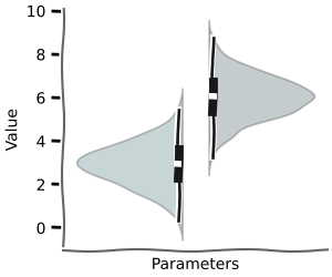
Steady-state¶

Using mc.steady_state you can calculate the steady-state distribution given the monte-carlo parameters.

This works analogously to the scan.steady_state function, except the index of the dataframes is always just an integer.

The parameters used can be obtained by result.parameters.

We will use a linear chain of reactions with two circles as an example model for this notebook.

$$ \begin{array}{c|c} \mathrm{Reaction} & \mathrm{Stoichiometry} \\ \hline v_0 & \varnothing \rightarrow{} \mathrm{x_1} \\ v_1 & -\mathrm{x_1} \rightarrow{} \mathrm{x_2} \\ v_2 & -\mathrm{x_1} \rightarrow{} \mathrm{x_3} \\ v_3 & -\mathrm{x_1} \rightarrow{} \mathrm{x_4} \\ v_4 & -\mathrm{x_4} \rightarrow{} \varnothing\\ v_5 & -\mathrm{x_2} \rightarrow{} \mathrm{x_1} \\ v_6 & -\mathrm{x_3} \rightarrow{} \mathrm{x_1} \\ \end{array} $$

In [3]:

ss = mc.steady_state(
    get_linear_chain_2v(),
    mc_to_scan=sample(
        {
            "k1": Uniform(0.9, 1.1),
            "k2": Uniform(1.0, 1.3),
            "k3": LogNormal(mean=1.0, sigma=0.2),
        },
        n=10,
    ),
)

fig, (ax1, ax2) = plot.two_axes(figsize=(6, 2.5), sharex=False)
plot.violins(ss.variables, ax=ax1)
plot.violins(ss.fluxes, ax=ax2)
ax1.set(xlabel="Variables", ylabel="Concentration / a.u.")
ax2.set(xlabel="Reactions", ylabel="Flux / a.u.")
plt.show()

ss = mc.steady_state( get_linear_chain_2v(), mc_to_scan=sample( { "k1": Uniform(0.9, 1.1), "k2": Uniform(1.0, 1.3), "k3": LogNormal(mean=1.0, sigma=0.2), }, n=10, ), ) fig, (ax1, ax2) = plot.two_axes(figsize=(6, 2.5), sharex=False) plot.violins(ss.variables, ax=ax1) plot.violins(ss.fluxes, ax=ax2) ax1.set(xlabel="Variables", ylabel="Concentration / a.u.") ax2.set(xlabel="Reactions", ylabel="Flux / a.u.") plt.show()

  0%|          | 0/10 [00:00<?, ?it/s]

 10%|█         | 1/10 [00:05<00:45,  5.10s/it]

 30%|███       | 3/10 [00:05<00:09,  1.38s/it]

100%|██████████| 10/10 [00:05<00:00,  3.29it/s]

100%|██████████| 10/10 [00:05<00:00,  1.87it/s]

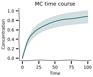
Time course¶

Using mc.time_course you can calculate time courses for sampled parameters.

+ =

This function works analogously to scan.time_course.

The pandas.DataFrames for concentrations and fluxes have a n x time pandas.MultiIndex.

The corresponding parameters can be found in result.parameters

In [4]:

tc = mc.time_course(
    get_linear_chain_2v(),
    time_points=np.linspace(0, 1, 11),
    mc_to_scan=sample(
        {
            "k1": Uniform(0.9, 1.1),
            "k2": Uniform(1.0, 1.3),
            "k3": LogNormal(mean=1.0, sigma=0.2),
        },
        n=10,
    ),
)

fig, (ax1, ax2) = plot.two_axes(figsize=(7, 4))
plot.lines_mean_std_from_2d_idx(tc.variables, ax=ax1)
plot.lines_mean_std_from_2d_idx(tc.fluxes, ax=ax2)
ax1.set(xlabel="Time / a.u", ylabel="Concentration / a.u.")
ax2.set(xlabel="Time / a.u", ylabel="Flux / a.u.")
plt.show()

tc = mc.time_course( get_linear_chain_2v(), time_points=np.linspace(0, 1, 11), mc_to_scan=sample( { "k1": Uniform(0.9, 1.1), "k2": Uniform(1.0, 1.3), "k3": LogNormal(mean=1.0, sigma=0.2), }, n=10, ), ) fig, (ax1, ax2) = plot.two_axes(figsize=(7, 4)) plot.lines_mean_std_from_2d_idx(tc.variables, ax=ax1) plot.lines_mean_std_from_2d_idx(tc.fluxes, ax=ax2) ax1.set(xlabel="Time / a.u", ylabel="Concentration / a.u.") ax2.set(xlabel="Time / a.u", ylabel="Flux / a.u.") plt.show()

  0%|          | 0/10 [00:00<?, ?it/s]

 10%|█         | 1/10 [00:04<00:44,  4.98s/it]

 50%|█████     | 5/10 [00:05<00:03,  1.28it/s]

100%|██████████| 10/10 [00:05<00:00,  1.93it/s]

Protocol time course¶

Using mc.time_course_over_protocol you can calculate time courses for sampled parameters given a discrete protocol.

+ =

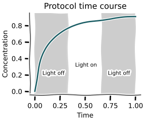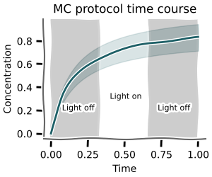
The pandas.DataFrames for concentrations and fluxes have a n x time pandas.MultiIndex.
The corresponding parameters can be found in scan.parameters

In [5]:

tc = mc.protocol_time_course(
    get_linear_chain_2v(),
    time_points=np.linspace(0, 6, 21),
    protocol=make_protocol(
        [
            (1, {"k1": 1}),
            (2, {"k1": 2}),
            (3, {"k1": 1}),
        ]
    ),
    mc_to_scan=sample(
        {
            "k2": Uniform(1.0, 1.3),
            "k3": LogNormal(mean=1.0, sigma=0.2),
        },
        n=10,
    ),
)

fig, (ax1, ax2) = plot.two_axes(figsize=(7, 4))
plot.lines_mean_std_from_2d_idx(tc.variables, ax=ax1)
plot.lines_mean_std_from_2d_idx(tc.fluxes, ax=ax2)
for ax in (ax1, ax2):
    plot.shade_protocol(tc.protocol["k1"], ax=ax, alpha=0.1)

ax1.set(xlabel="Time / a.u", ylabel="Concentration / a.u.")
ax2.set(xlabel="Time / a.u", ylabel="Flux / a.u.")
plt.show()

tc = mc.protocol_time_course( get_linear_chain_2v(), time_points=np.linspace(0, 6, 21), protocol=make_protocol( [ (1, {"k1": 1}), (2, {"k1": 2}), (3, {"k1": 1}), ] ), mc_to_scan=sample( { "k2": Uniform(1.0, 1.3), "k3": LogNormal(mean=1.0, sigma=0.2), }, n=10, ), ) fig, (ax1, ax2) = plot.two_axes(figsize=(7, 4)) plot.lines_mean_std_from_2d_idx(tc.variables, ax=ax1) plot.lines_mean_std_from_2d_idx(tc.fluxes, ax=ax2) for ax in (ax1, ax2): plot.shade_protocol(tc.protocol["k1"], ax=ax, alpha=0.1) ax1.set(xlabel="Time / a.u", ylabel="Concentration / a.u.") ax2.set(xlabel="Time / a.u", ylabel="Flux / a.u.") plt.show()

  0%|          | 0/10 [00:00<?, ?it/s]

  0%|          | 0/10 [00:04<?, ?it/s]

---------------------------------------------------------------------------
_RemoteTraceback                          Traceback (most recent call last)
_RemoteTraceback: 
"""
Traceback (most recent call last):
  File "/home/runner/work/MxlPy/MxlPy/.venv/lib/python3.13/site-packages/loky/process_executor.py", line 490, in _process_worker
    r = call_item()
  File "/home/runner/work/MxlPy/MxlPy/.venv/lib/python3.13/site-packages/loky/process_executor.py", line 291, in __call__
    return self.fn(*self.args, **self.kwargs)
           ~~~~~~~^^^^^^^^^^^^^^^^^^^^^^^^^^^
  File "/home/runner/work/MxlPy/MxlPy/src/mxlpy/parallel.py", line 94, in _load_or_run
    res = fn(v)
  File "/home/runner/work/MxlPy/MxlPy/src/mxlpy/scan.py", line 80, in _update_parameters_and_initial_conditions
    return fn(model)
  File "/home/runner/work/MxlPy/MxlPy/src/mxlpy/scan.py", line 315, in _protocol_time_course_worker
    .simulate_protocol_time_course(
     ~~~~~~~~~~~~~~~~~~~~~~~~~~~~~^
        protocol=protocol,
        ^^^^^^^^^^^^^^^^^^
        time_points=time_points,
        ^^^^^^^^^^^^^^^^^^^^^^^^
    )
    ^
  File "/home/runner/work/MxlPy/MxlPy/src/mxlpy/simulator.py", line 548, in simulate_protocol_time_course
    self.model.update_parameters(cast(dict, pars.to_dict()))
    ~~~~~~~~~~~~~~~~~~~~~~~~~~~~^^^^^^^^^^^^^^^^^^^^^^^^^^^^
  File "/home/runner/work/MxlPy/MxlPy/src/mxlpy/model.py", line 784, in update_parameters
    self.update_parameter(k, v)
    ~~~~~~~~~~~~~~~~~~~~~^^^^^^
  File "/home/runner/work/MxlPy/MxlPy/src/mxlpy/model.py", line 207, in wrapper
    return method(*args, **kwargs)
  File "/home/runner/work/MxlPy/MxlPy/src/mxlpy/model.py", line 749, in update_parameter
    raise KeyError(msg)
KeyError: "Parameter 'k1' not found. Available parameters: ['k2', 'k_in', 'k_out']"
"""

The above exception was the direct cause of the following exception:

KeyError                                  Traceback (most recent call last)
Cell In[5], line 1
----> 1 tc = mc.protocol_time_course(
      2     get_linear_chain_2v(),
      3     time_points=np.linspace(0, 6, 21),
      4     protocol=make_protocol(

File ~/work/MxlPy/MxlPy/src/mxlpy/mc.py:427, in protocol_time_course(model, protocol, time_points, mc_to_scan, y0, max_workers, cache, worker, integrator)
    424 if y0 is not None:
    425     model.update_variables(y0)
--> 427 res = parallelise(
    428     partial(
    429         _update_parameters_and_initial_conditions,
    430         fn=partial(
    431             worker,
    432             protocol=protocol,
    433             time_points=time_points,
    434             integrator=integrator,
    435             y0=None,
    436         ),
    437         model=model,
    438     ),
    439     inputs=list(mc_to_scan.iterrows()),
    440     max_workers=max_workers,
    441     cache=cache,
    442 )
    443 return ProtocolScan(
    444     to_scan=mc_to_scan,
    445     protocol=protocol,
    446     raw_results=dict(res),
    447 )

File ~/work/MxlPy/MxlPy/src/mxlpy/parallel.py:173, in parallelise(fn, inputs, cache, parallel, max_workers, timeout, disable_tqdm, tqdm_desc)
    171 for future in futures:
    172     try:
--> 173         key, value = future.result(timeout=timeout)
    174         pbar.update(1)
    175         results.append((key, value))

File ~/.local/share/uv/python/cpython-3.13.12-linux-x86_64-gnu/lib/python3.13/concurrent/futures/_base.py:456, in Future.result(self, timeout)
    454     raise CancelledError()
    455 elif self._state == FINISHED:
--> 456     return self.__get_result()
    457 else:
    458     raise TimeoutError()

File ~/.local/share/uv/python/cpython-3.13.12-linux-x86_64-gnu/lib/python3.13/concurrent/futures/_base.py:401, in Future.__get_result(self)
    399 if self._exception is not None:
    400     try:
--> 401         raise self._exception
    402     finally:
    403         # Break a reference cycle with the exception in self._exception
    404         self = None

KeyError: "Parameter 'k1' not found. Available parameters: ['k2', 'k_in', 'k_out']"

Metabolic control analysis¶

mxlpy further has routines for monte-carlo distributed metabolic control analysis.
This allows quantifying, whether the coefficients obtained from the MCA analysis are robust against parameter changes or whether they are just an artifact of a particular choice of parameters.

Variable elasticities¶

+ =

The returned pandas.DataFrame has a pd.MultiIndex of shape n x reaction.

In [6]:

mc_elas = mc.variable_elasticities(
    get_upper_glycolysis(),
    variables={
        "GLC": 0.3,
        "G6P": 0.4,
        "F6P": 0.5,
        "FBP": 0.6,
        "ATP": 0.4,
        "ADP": 0.6,
    },
    to_scan=["GLC", "F6P"],
    mc_to_scan=sample(
        {
            # "k1": LogNormal(mean=np.log(0.25), sigma=1.0),
            # "k2": LogNormal(mean=np.log(1.0), sigma=1.0),
            "k3": LogNormal(mean=np.log(1.0), sigma=1.0),
            # "k4": LogNormal(mean=np.log(1.0), sigma=1.0),
            # "k5": LogNormal(mean=np.log(1.0), sigma=1.0),
            # "k6": LogNormal(mean=np.log(1.0), sigma=1.0),
            # "k7": LogNormal(mean=np.log(2.5), sigma=1.0),
        },
        n=5,
    ),
)

_ = plot.violins_from_2d_idx(mc_elas)
plt.show()

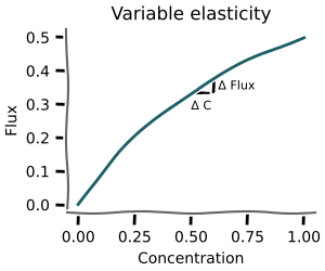
mc_elas = mc.variable_elasticities( get_upper_glycolysis(), variables={ "GLC": 0.3, "G6P": 0.4, "F6P": 0.5, "FBP": 0.6, "ATP": 0.4, "ADP": 0.6, }, to_scan=["GLC", "F6P"], mc_to_scan=sample( { # "k1": LogNormal(mean=np.log(0.25), sigma=1.0), # "k2": LogNormal(mean=np.log(1.0), sigma=1.0), "k3": LogNormal(mean=np.log(1.0), sigma=1.0), # "k4": LogNormal(mean=np.log(1.0), sigma=1.0), # "k5": LogNormal(mean=np.log(1.0), sigma=1.0), # "k6": LogNormal(mean=np.log(1.0), sigma=1.0), # "k7": LogNormal(mean=np.log(2.5), sigma=1.0), }, n=5, ), ) _ = plot.violins_from_2d_idx(mc_elas) plt.show()

  0%|          | 0/5 [00:00<?, ?it/s]

 20%|██        | 1/5 [00:04<00:19,  4.97s/it]

 40%|████      | 2/5 [00:05<00:06,  2.11s/it]

100%|██████████| 5/5 [00:05<00:00,  1.61it/s]

100%|██████████| 5/5 [00:05<00:00,  1.03s/it]

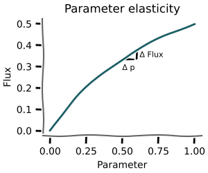
Parameter elasticities¶

+ =

In [7]:

elas = mc.parameter_elasticities(
    get_upper_glycolysis(),
    variables={
        "GLC": 0.3,
        "G6P": 0.4,
        "F6P": 0.5,
        "FBP": 0.6,
        "ATP": 0.4,
        "ADP": 0.6,
    },
    to_scan=["k1", "k2", "k3"],
    mc_to_scan=sample(
        {
            "k3": LogNormal(mean=np.log(0.25), sigma=1.0),
        },
        n=5,
    ),
)

_ = plot.violins_from_2d_idx(elas)
plt.show()

elas = mc.parameter_elasticities( get_upper_glycolysis(), variables={ "GLC": 0.3, "G6P": 0.4, "F6P": 0.5, "FBP": 0.6, "ATP": 0.4, "ADP": 0.6, }, to_scan=["k1", "k2", "k3"], mc_to_scan=sample( { "k3": LogNormal(mean=np.log(0.25), sigma=1.0), }, n=5, ), ) _ = plot.violins_from_2d_idx(elas) plt.show()

  0%|          | 0/5 [00:00<?, ?it/s]

 20%|██        | 1/5 [00:04<00:19,  5.00s/it]

 40%|████      | 2/5 [00:05<00:06,  2.14s/it]

100%|██████████| 5/5 [00:05<00:00,  1.05s/it]

Response coefficients¶

+ =

In [8]:

# Compare with "normal" control coefficients
rc = mca.response_coefficients(
    get_lin_chain_two_circles(),
    to_scan=["vmax_1", "vmax_2", "vmax_3", "vmax_5", "vmax_6"],
)
_ = plot.heatmap(rc.variables)

mrc = mc.response_coefficients(
    get_lin_chain_two_circles(),
    to_scan=["vmax_1", "vmax_2", "vmax_3", "vmax_5", "vmax_6"],
    mc_to_scan=sample(
        {
            "k0": LogNormal(np.log(1.0), 1.0),
            "k4": LogNormal(np.log(0.5), 1.0),
        },
        n=10,
    ),
)

_ = plot.violins_from_2d_idx(mrc.variables, n_cols=len(mrc.variables.columns))

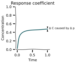# Compare with "normal" control coefficients rc = mca.response_coefficients( get_lin_chain_two_circles(), to_scan=["vmax_1", "vmax_2", "vmax_3", "vmax_5", "vmax_6"], ) _ = plot.heatmap(rc.variables) mrc = mc.response_coefficients( get_lin_chain_two_circles(), to_scan=["vmax_1", "vmax_2", "vmax_3", "vmax_5", "vmax_6"], mc_to_scan=sample( { "k0": LogNormal(np.log(1.0), 1.0), "k4": LogNormal(np.log(0.5), 1.0), }, n=10, ), ) _ = plot.violins_from_2d_idx(mrc.variables, n_cols=len(mrc.variables.columns))

  0%|          | 0/5 [00:00<?, ?it/s]

 20%|██        | 1/5 [00:05<00:20,  5.03s/it]

100%|██████████| 5/5 [00:05<00:00,  1.25it/s]

100%|██████████| 5/5 [00:05<00:00,  1.06s/it]

  0%|          | 0/10 [00:00<?, ?it/s]

  0%|          | 0/5 [00:00<?, ?it/s]
  0%|          | 0/5 [00:00<?, ?it/s]
  0%|          | 0/5 [00:00<?, ?it/s]
  0%|          | 0/5 [00:00<?, ?it/s]
 40%|████      | 2/5 [00:00<00:00, 11.87it/s]

 40%|████      | 2/5 [00:00<00:00, 10.26it/s]
 40%|████      | 2/5 [00:00<00:00, 12.49it/s]
 80%|████████  | 4/5 [00:00<00:00, 12.34it/s]
100%|██████████| 5/5 [00:00<00:00, 12.28it/s]
 10%|█         | 1/10 [00:05<00:48,  5.44s/it]

 80%|████████  | 4/5 [00:00<00:00, 10.45it/s]
 80%|████████  | 4/5 [00:00<00:00, 12.41it/s]

100%|██████████| 5/5 [00:00<00:00, 10.83it/s]

100%|██████████| 5/5 [00:00<00:00, 12.45it/s]

  0%|          | 0/5 [00:00<?, ?it/s]

  0%|          | 0/5 [00:00<?, ?it/s]
  0%|          | 0/5 [00:00<?, ?it/s]

 40%|████      | 2/5 [00:00<00:00, 13.43it/s]
 40%|████      | 2/5 [00:00<00:00, 10.25it/s]

 80%|████████  | 4/5 [00:00<00:00, 11.99it/s]

100%|██████████| 5/5 [00:00<00:00, 11.94it/s]

  0%|          | 0/5 [00:00<?, ?it/s]
 80%|████████  | 4/5 [00:00<00:00, 10.27it/s]

 40%|████      | 2/5 [00:00<00:00, 12.40it/s]
100%|██████████| 5/5 [00:00<00:00, 10.26it/s]

  0%|          | 0/5 [00:00<?, ?it/s]

 80%|████████  | 4/5 [00:00<00:00, 12.26it/s]
 40%|████      | 2/5 [00:00<00:00, 10.86it/s]

100%|██████████| 5/5 [00:00<00:00, 12.25it/s]

  0%|          | 0/5 [00:00<?, ?it/s]

 80%|████████  | 4/5 [00:00<00:00, 10.85it/s]
 40%|████      | 2/5 [00:00<00:00, 11.92it/s]

100%|██████████| 5/5 [00:00<00:00, 10.88it/s]

 80%|████████  | 4/5 [00:00<00:00, 12.11it/s]
100%|██████████| 5/5 [00:00<00:00, 12.13it/s]

 20%|██        | 1/5 [00:04<00:16,  4.11s/it]

 20%|██        | 1/5 [00:03<00:15,  3.95s/it]

 40%|████      | 2/5 [00:07<00:11,  3.69s/it]

 40%|████      | 2/5 [00:07<00:10,  3.63s/it]

 60%|██████    | 3/5 [00:10<00:07,  3.55s/it]

 60%|██████    | 3/5 [00:10<00:07,  3.53s/it]

 80%|████████  | 4/5 [00:14<00:03,  3.49s/it]

 80%|████████  | 4/5 [00:14<00:03,  3.48s/it]

100%|██████████| 5/5 [00:17<00:00,  3.46s/it]
100%|██████████| 5/5 [00:17<00:00,  3.54s/it]

 40%|████      | 4/10 [00:22<00:34,  5.74s/it]

100%|██████████| 5/5 [00:17<00:00,  3.45s/it]
100%|██████████| 5/5 [00:17<00:00,  3.51s/it]

 60%|██████    | 6/10 [00:23<00:13,  3.33s/it]

100%|██████████| 10/10 [00:23<00:00,  2.33s/it]

First finish line

With that you now know most of what you will need from a day-to-day basis about monte carlo methods in mxlpy.

Congratulations!

Advanced topics¶

Parameter scans¶

Vary both monte carlo parameters as well as systematically scan for other parameters

In [9]:

mcss = mc.scan_steady_state(
    get_linear_chain_2v(),
    to_scan=pd.DataFrame({"k1": np.linspace(0, 1, 3)}),
    mc_to_scan=sample(
        {
            "k2": Uniform(1.0, 1.3),
            "k3": LogNormal(mean=1.0, sigma=0.2),
        },
        n=10,
    ),
)

plot.violins_from_2d_idx(mcss.variables)
plt.show()

mcss = mc.scan_steady_state( get_linear_chain_2v(), to_scan=pd.DataFrame({"k1": np.linspace(0, 1, 3)}), mc_to_scan=sample( { "k2": Uniform(1.0, 1.3), "k3": LogNormal(mean=1.0, sigma=0.2), }, n=10, ), ) plot.violins_from_2d_idx(mcss.variables) plt.show()

  0%|          | 0/10 [00:00<?, ?it/s]

  0%|          | 0/3 [00:00<?, ?it/s]
  0%|          | 0/3 [00:00<?, ?it/s]
100%|██████████| 3/3 [00:00<00:00, 165.72it/s]

 10%|█         | 1/10 [00:04<00:44,  5.00s/it]

  0%|          | 0/3 [00:00<?, ?it/s]
100%|██████████| 3/3 [00:00<00:00, 151.86it/s]

  0%|          | 0/3 [00:00<?, ?it/s]
100%|██████████| 3/3 [00:00<00:00, 173.57it/s]

100%|██████████| 3/3 [00:00<00:00, 211.34it/s]

  0%|          | 0/3 [00:00<?, ?it/s]
  0%|          | 0/3 [00:00<?, ?it/s]
100%|██████████| 3/3 [00:00<00:00, 269.41it/s]

  0%|          | 0/3 [00:00<?, ?it/s]
 50%|█████     | 5/10 [00:05<00:03,  1.27it/s]

  0%|          | 0/3 [00:00<?, ?it/s]
  0%|          | 0/3 [00:00<?, ?it/s]
100%|██████████| 3/3 [00:00<00:00, 204.04it/s]

  0%|          | 0/3 [00:00<?, ?it/s]
100%|██████████| 3/3 [00:00<00:00, 208.80it/s]

100%|██████████| 3/3 [00:00<00:00, 238.98it/s]

100%|██████████| 3/3 [00:00<00:00, 172.42it/s]

100%|██████████| 3/3 [00:00<00:00, 185.75it/s]

100%|██████████| 10/10 [00:05<00:00,  1.91it/s]

INFO:matplotlib.category:Using categorical units to plot a list of strings that are all parsable as floats or dates. If these strings should be plotted as numbers, cast to the appropriate data type before plotting.

INFO:matplotlib.category:Using categorical units to plot a list of strings that are all parsable as floats or dates. If these strings should be plotted as numbers, cast to the appropriate data type before plotting.

INFO:matplotlib.category:Using categorical units to plot a list of strings that are all parsable as floats or dates. If these strings should be plotted as numbers, cast to the appropriate data type before plotting.

INFO:matplotlib.category:Using categorical units to plot a list of strings that are all parsable as floats or dates. If these strings should be plotted as numbers, cast to the appropriate data type before plotting.

In [10]:

# FIXME: no idea how to plot this yet. Ridge plots?
# Maybe it's just a bit much :D

mcss = mc.scan_steady_state(
    get_linear_chain_2v(),
    to_scan=mb2.cartesian_product(
        {
            "k1": np.linspace(0, 1, 3),
            "k2": np.linspace(0, 1, 3),
        }
    ),
    mc_to_scan=sample(
        {
            "k3": LogNormal(mean=1.0, sigma=0.2),
        },
        n=10,
    ),
)

mcss.variables.head()

# FIXME: no idea how to plot this yet. Ridge plots? # Maybe it's just a bit much :D mcss = mc.scan_steady_state( get_linear_chain_2v(), to_scan=mb2.cartesian_product( { "k1": np.linspace(0, 1, 3), "k2": np.linspace(0, 1, 3), } ), mc_to_scan=sample( { "k3": LogNormal(mean=1.0, sigma=0.2), }, n=10, ), ) mcss.variables.head()

  0%|          | 0/10 [00:00<?, ?it/s]

  0%|          | 0/9 [00:00<?, ?it/s]
  0%|          | 0/9 [00:00<?, ?it/s]
  0%|          | 0/9 [00:00<?, ?it/s]
  0%|          | 0/9 [00:00<?, ?it/s]

 11%|█         | 1/9 [00:00<00:06,  1.33it/s]
 11%|█         | 1/9 [00:00<00:06,  1.32it/s]
 11%|█         | 1/9 [00:00<00:06,  1.29it/s]
 11%|█         | 1/9 [00:00<00:06,  1.28it/s]

 44%|████▍     | 4/9 [00:01<00:01,  2.88it/s]
 44%|████▍     | 4/9 [00:01<00:01,  2.87it/s]
 44%|████▍     | 4/9 [00:01<00:01,  2.80it/s]
 44%|████▍     | 4/9 [00:01<00:01,  2.80it/s]

 78%|███████▊  | 7/9 [00:02<00:00,  3.36it/s]
 78%|███████▊  | 7/9 [00:02<00:00,  3.35it/s]
100%|██████████| 9/9 [00:02<00:00,  3.94it/s]

100%|██████████| 9/9 [00:02<00:00,  3.93it/s]

 78%|███████▊  | 7/9 [00:02<00:00,  3.29it/s]
100%|██████████| 9/9 [00:02<00:00,  3.85it/s]

 10%|█         | 1/10 [00:07<01:06,  7.34s/it]

 78%|███████▊  | 7/9 [00:02<00:00,  3.31it/s]
100%|██████████| 9/9 [00:02<00:00,  3.87it/s]

  0%|          | 0/9 [00:00<?, ?it/s]
  0%|          | 0/9 [00:00<?, ?it/s]
  0%|          | 0/9 [00:00<?, ?it/s]
  0%|          | 0/9 [00:00<?, ?it/s]

 11%|█         | 1/9 [00:00<00:06,  1.30it/s]
 11%|█         | 1/9 [00:00<00:06,  1.27it/s]
 11%|█         | 1/9 [00:00<00:05,  1.36it/s]
 11%|█         | 1/9 [00:00<00:06,  1.26it/s]

 44%|████▍     | 4/9 [00:01<00:01,  2.81it/s]
 44%|████▍     | 4/9 [00:01<00:01,  2.86it/s]
 44%|████▍     | 4/9 [00:01<00:01,  2.77it/s]
 44%|████▍     | 4/9 [00:01<00:01,  2.78it/s]

 78%|███████▊  | 7/9 [00:02<00:00,  3.29it/s]
100%|██████████| 9/9 [00:02<00:00,  3.86it/s]

  0%|          | 0/9 [00:00<?, ?it/s]
 50%|█████     | 5/10 [00:09<00:08,  1.62s/it]

 78%|███████▊  | 7/9 [00:02<00:00,  3.32it/s]
 78%|███████▊  | 7/9 [00:02<00:00,  3.27it/s]
100%|██████████| 9/9 [00:02<00:00,  3.91it/s]

100%|██████████| 9/9 [00:02<00:00,  3.82it/s]

  0%|          | 0/9 [00:00<?, ?it/s]
 78%|███████▊  | 7/9 [00:02<00:00,  3.27it/s]
100%|██████████| 9/9 [00:02<00:00,  3.82it/s]

 11%|█         | 1/9 [00:00<00:03,  2.38it/s]
 11%|█         | 1/9 [00:00<00:03,  2.31it/s]

 44%|████▍     | 4/9 [00:00<00:00,  5.32it/s]
 44%|████▍     | 4/9 [00:00<00:00,  5.25it/s]

 78%|███████▊  | 7/9 [00:01<00:00,  6.26it/s]
100%|██████████| 9/9 [00:01<00:00,  7.30it/s]

 90%|█████████ | 9/10 [00:11<00:00,  1.11it/s]

 78%|███████▊  | 7/9 [00:01<00:00,  6.21it/s]
100%|██████████| 9/9 [00:01<00:00,  7.22it/s]

100%|██████████| 10/10 [00:11<00:00,  1.11s/it]

Out[10]:

			x	y
	k1	k2
0	0.0	0.0	NaN	NaN
		0.5	2.0	1.0
		1.0	1.0	1.0
	0.5	0.0	NaN	NaN
		0.5	2.0	1.0

Custom distributions¶

If you want to create custom distributions, all you need to do is to create a class that follows the Distribution protocol, e.g. implements a sample function.

For API consistency, the sample method has to take rng argument, which can be ignored if not applicable.

In [11]:

from dataclasses import dataclass
from typing import TYPE_CHECKING

if TYPE_CHECKING:
    from mxlpy.types import Array


@dataclass
class MyOwnDistribution:
    loc: float = 0.0
    scale: float = 1.0

    def sample(
        self,
        num: int,
        rng: np.random.Generator | None = None,
    ) -> Array:
        if rng is None:
            rng = np.random.default_rng()
        return rng.normal(loc=self.loc, scale=self.scale, size=num)


sample({"p1": MyOwnDistribution()}, n=5)

from dataclasses import dataclass from typing import TYPE_CHECKING if TYPE_CHECKING: from mxlpy.types import Array @dataclass class MyOwnDistribution: loc: float = 0.0 scale: float = 1.0 def sample( self, num: int, rng: np.random.Generator | None = None, ) -> Array: if rng is None: rng = np.random.default_rng() return rng.normal(loc=self.loc, scale=self.scale, size=num) sample({"p1": MyOwnDistribution()}, n=5)

Out[11]:

	p1
0	0.834082
1	-0.146356
2	-0.080290
3	-2.393945
4	-0.236137

In [ ]: