from __future__ import annotations

import matplotlib.pyplot as plt

from example_models import get_upper_glycolysis
from mxlpy import plot
Metabolic control analysis
Metabolic control analysis answers the question: what happens to the concentrations and fluxes if I slightly perturb the system?
It is thus a local measurement about which reactions hold the most control.
The most common measurements are elasticities and response coefficients.
The main difference between them is that response coefficients are calculated at steady-state, while elasticities can be calculated at every arbitrary state.
All the required functionality can be found in the mxlpy.mca module.
As an example, we will use the upper glycolysis model from the Systems Biology textbook by Klipp et al. (2005).
from mxlpy import mca
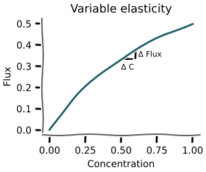
Variable elasticities
Variable elasticities are the sensitivity of reactions to a small change in the concentration of a variable.
They are not a steady-state measurement and can be calculated for any arbitrary state.
Both the concs and variables arguments are optional.
If concs is not supplied, the routine will use the initial conditions from the model.
If variables is not supplied, the elasticities will be calculated for all variables.
elas = mca.variable_elasticities(
    get_upper_glycolysis(),
    to_scan=["GLC", "F6P"],
    variables={
        "GLC": 0.3,
        "G6P": 0.4,
        "F6P": 0.5,
        "FBP": 0.6,
        "ATP": 0.4,
        "ADP": 0.6,
    },
)

_ = plot.heatmap(elas)
plt.show()

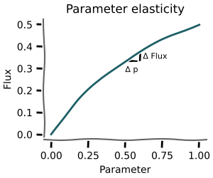
Parameter elasticities
Similarly, parameter elasticities are the sensitivity of reactions to a small change in the concentration of a variable.
They are not a steady-state measurement and can be calculated for any arbitrary state.
Both the concs and parameters arguments are optional.
If concs is not supplied, the routine will use the initial conditions from the model.
If parameters is not supplied, the elasticities will be calculated for all parameters.
elas = mca.parameter_elasticities(
    get_upper_glycolysis(),
    variables={
        "GLC": 0.3,
        "G6P": 0.4,
        "F6P": 0.5,
        "FBP": 0.6,
        "ATP": 0.4,
        "ADP": 0.6,
    },
    to_scan=["k1", "k2"],
)

_ = plot.heatmap(elas)
plt.show()

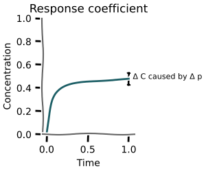
Response coefficients
Response coefficients show the sensitivity of variables and reactions at steady-state to a small change in a parameter.
If the parameter is proportional to the rate, they are also called control coefficients.
Calculation of these is run in parallel by default.
crcs, frcs = mca.response_coefficients(
    get_upper_glycolysis(),
    to_scan=["k1", "k2", "k3", "k4", "k5", "k6", "k7"],
)

fig, (ax1, ax2) = plt.subplots(1, 2, figsize=(12, 4))
_ = plot.heatmap(crcs, ax=ax1)
_ = plot.heatmap(frcs, ax=ax2)
plt.show()
0%| | 0/7 [00:00<?, ?it/s]
14%|█▍ | 1/7 [00:05<00:34, 5.73s/it]
57%|█████▋ | 4/7 [00:05<00:03, 1.12s/it]
100%|██████████| 7/7 [00:05<00:00, 1.86it/s]
100%|██████████| 7/7 [00:05<00:00, 1.17it/s]

Steady-state stability
After finding a steady state you can classify its local stability from the eigenvalues of the Jacobian.
steady_state_stability evaluates the symbolic Jacobian at the given state, computes eigenvalues with numpy.linalg.eigvals, and returns a SteadyStateStability object:
| Field | Description |
|---|---|
eigenvalues |
Complex Jacobian eigenvalues |
spectral_abscissa |
Largest real part — negative ⟺ stable |
is_stable |
True when all real parts are negative |
has_oscillatory |
True when any eigenvalue has nonzero imaginary part |
classification |
"stable node" | "stable spiral" | "unstable node" | "unstable spiral" | "saddle point" | "centre" | "non-hyperbolic" |
from mxlpy import Simulator
from mxlpy.mca import steady_state_stability

model = get_upper_glycolysis()
ss = (
    Simulator(model)
    .simulate_to_steady_state()
    .get_result()
    .unwrap_or_err()
    .get_new_y0()
)

stab = steady_state_stability(model, ss)
print(f"Classification : {stab.classification}")
print(f"Is stable      : {stab.is_stable}")
print(f"Spectral absc. : {stab.spectral_abscissa:.4f}")
print(f"Has oscillatory: {stab.has_oscillatory}")
print(f"Eigenvalues    : {stab.eigenvalues}")
Classification : non-hyperbolic
Is stable      : False
Spectral absc. : -0.0000
Has oscillatory: False
Eigenvalues    : [-4.11651781e+00+1.18855663e-17j -1.10480692e-01+5.10294300e-19j -6.83582444e-01-4.54290092e-20j -1.60342820e+00+0.00000000e+00j -2.45741943e+00+0.00000000e+00j -1.11022302e-16+0.00000000e+00j]
Supply-demand rate characteristics
Where the analyses above are local (a small perturbation around a single state), rate characteristics show the global picture: how the reactions that produce and consume a metabolite respond across its whole concentration range.
rate_characteristics clamps a chosen variable to a logarithmically spaced range around its steady-state concentration, recomputes the steady state of the remaining variables at each point, and collects the fluxes of the reactions that produce it (supply) and consume it (demand). The intersection of total supply and total demand is the steady state — plotting both curves places that operating point in the context of the full range.
Reactions are classified structurally from the stoichiometry: a positive coefficient marks a supply reaction, a negative one a demand reaction. The scan spans [ss / min_factor, ss * max_factor] with n_points log-spaced samples.
The result exposes:
| Attribute / method | Description |
|---|---|
supply_fluxes / demand_fluxes |
Per-reaction fluxes vs. the clamped concentration (one column per reaction) |
total_supply / total_demand |
Summed supply / demand flux |
steady_state_conc |
Concentration of the variable at the original steady state |
plot_supply_demand() |
Total supply and demand on a single log-log axis |
plot() |
Three-panel summary: total supply vs. demand, per-reaction supply, per-reaction demand |
Here we scan F6P, which is produced by two reactions (v3, v5) and consumed by one (v4).
rc = mca.rate_characteristics(get_upper_glycolysis(), "F6P")

_ = rc.plot()
plt.show()
0%| | 0/256 [00:00<?, ?it/s]
0%| | 1/256 [00:05<23:13, 5.46s/it]
2%|▏ | 5/256 [00:05<03:36, 1.16it/s]
9%|▊ | 22/256 [00:05<00:33, 6.91it/s]
19%|█▉ | 49/256 [00:05<00:10, 19.11it/s]
30%|██▉ | 76/256 [00:05<00:05, 34.62it/s]
41%|████ | 104/256 [00:06<00:02, 54.48it/s]
50%|█████ | 129/256 [00:06<00:01, 74.59it/s]
59%|█████▉ | 152/256 [00:06<00:01, 93.76it/s]
68%|██████▊ | 175/256 [00:06<00:00, 110.03it/s]
77%|███████▋ | 197/256 [00:06<00:00, 120.51it/s]
85%|████████▍ | 217/256 [00:06<00:00, 123.37it/s]
92%|█████████▏| 235/256 [00:06<00:00, 116.05it/s]
98%|█████████▊| 251/256 [00:07<00:00, 108.60it/s]
100%|██████████| 256/256 [00:07<00:00, 35.89it/s]

First finish line
With that you now know most of what you will need from a day-to-day basis about metabolic control analysis in mxlpy.Congratulations!
Advanced concepts / customisation
Normalisation
By default the elasticities and response coefficients are normalised, so e.g. for the response coefficients the following is calculated:
$$C^J_{v_i} = \left( \frac{dJ}{dp} \frac{p}{J} \right) \bigg/ \left( \frac{\partial v_i}{\partial p}\frac{p}{v_i} \right)$$
You can also obtain the non-normalised coefficients, by setting normalized=False, which amounts to the following calculation:
$$C^J_{v_i} = \left( \frac{dJ}{dp} \frac{p}{J} \right)$$
_ = mca.response_coefficients(
    get_upper_glycolysis(),
    to_scan=["k1", "k2", "k3", "k4", "k5", "k6", "k7"],
    normalized=False,
)
0%| | 0/7 [00:00<?, ?it/s]
14%|█▍ | 1/7 [00:05<00:32, 5.39s/it]
71%|███████▏ | 5/7 [00:05<00:01, 1.21it/s]
100%|██████████| 7/7 [00:05<00:00, 1.26it/s]
Displacement
We wrote above that we slightly change the value, but by how much exactly?
By default the relative change is set to 1e-4.
mxlpy uses a central finite difference approximation, which means that in this case change the value to
$$\textrm{value} \cdot \left(1 \pm 10^{-4} \right)$$
which amounts to a change of 0.01 %.
You can set that using the displacement argument.
_ = mca.response_coefficients(
    get_upper_glycolysis(),
    to_scan=["k1", "k2", "k3", "k4", "k5", "k6", "k7"],
    displacement=1e-2,
)
0%| | 0/7 [00:00<?, ?it/s]
14%|█▍ | 1/7 [00:05<00:32, 5.45s/it]
29%|██▊ | 2/7 [00:05<00:12, 2.43s/it]
100%|██████████| 7/7 [00:05<00:00, 2.06it/s]
100%|██████████| 7/7 [00:05<00:00, 1.19it/s]