Numerical parameter identifiability¶

See the course by Marisa Eisenberg for an excellent introduction into the topic

In [1]:

import numpy as np

from mxlpy import Model, Simulator, fns, plot
from mxlpy.identify import profile_likelihood

import numpy as np from mxlpy import Model, Simulator, fns, plot from mxlpy.identify import profile_likelihood

We start with an SIR model, which we use to generate some data (this would usually be experimentally measured data)

In [2]:

def sir() -> Model:
    return (
        Model()
        .add_variables({"s": 0.9, "i": 0.1, "r": 0.0})
        .add_parameters({"beta": 0.2, "gamma": 0.1})
        .add_reaction(
            "infection",
            fns.mass_action_2s,
            args=["s", "i", "beta"],
            stoichiometry={"s": -1, "i": 1},
        )
        .add_reaction(
            "recovery",
            fns.mass_action_1s,
            args=["i", "gamma"],
            stoichiometry={"i": -1, "r": 1},
        )
    )


data = Simulator(sir()).simulate(100).get_result().unwrap_or_err().variables
_ = plot.lines(data)

def sir() -> Model: return ( Model() .add_variables({"s": 0.9, "i": 0.1, "r": 0.0}) .add_parameters({"beta": 0.2, "gamma": 0.1}) .add_reaction( "infection", fns.mass_action_2s, args=["s", "i", "beta"], stoichiometry={"s": -1, "i": 1}, ) .add_reaction( "recovery", fns.mass_action_1s, args=["i", "gamma"], stoichiometry={"i": -1, "r": 1}, ) ) data = Simulator(sir()).simulate(100).get_result().unwrap_or_err().variables _ = plot.lines(data)

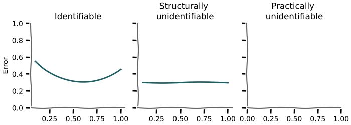
We then, for n different values of each parameter we are interested in, we

• draw random samples for the remaining model parameters
• fit the model to the data (excluding the parameter we are interested in) and note the final error
• visualise the error for each parameter value

The error for a parameter should show a clear minimum around the different values used, otherwise it is not identifiable

In [3]:

errors_beta = profile_likelihood(
    sir(),
    data=data,
    parameter_name="beta",
    parameter_values=np.linspace(0.2 * 0.5, 0.2 * 1.5, 10),
    n_random=10,
)

fig, ax = plot.lines(errors_beta, legend=False)
ax.set(title="beta", xlabel="parameter value", ylabel="abs(error)")
plot.show()

errors_beta = profile_likelihood( sir(), data=data, parameter_name="beta", parameter_values=np.linspace(0.2 * 0.5, 0.2 * 1.5, 10), n_random=10, ) fig, ax = plot.lines(errors_beta, legend=False) ax.set(title="beta", xlabel="parameter value", ylabel="abs(error)") plot.show()

beta:   0%|          | 0/10 [00:00<?, ?it/s]

beta:  10%|█         | 1/10 [00:07<01:04,  7.20s/it]

beta:  20%|██        | 2/10 [00:14<00:55,  6.97s/it]

beta:  30%|███       | 3/10 [00:21<00:48,  6.99s/it]

beta:  40%|████      | 4/10 [00:27<00:41,  6.95s/it]

beta:  50%|█████     | 5/10 [00:35<00:35,  7.04s/it]

beta:  60%|██████    | 6/10 [00:42<00:28,  7.03s/it]

beta:  70%|███████   | 7/10 [00:49<00:21,  7.05s/it]

beta:  80%|████████  | 8/10 [00:56<00:13,  7.00s/it]

beta:  90%|█████████ | 9/10 [01:02<00:06,  6.85s/it]

beta: 100%|██████████| 10/10 [01:09<00:00,  6.77s/it]

beta: 100%|██████████| 10/10 [01:09<00:00,  6.92s/it]