Neural Posterior Estimation

In [1]:

from __future__ import annotations

from functools import partial

import matplotlib.pyplot as plt
import numpy as np
import optax
import pandas as pd
import seaborn as sns
from numpy.polynomial.polynomial import Polynomial

from example_models.linear_chain import get_linear_chain_2v
from mxlpy import Model, Simulator, SurrogateProtocol, fns, npe, plot, scan, surrogates
from mxlpy.distributions import LogNormal, Normal, sample

from __future__ import annotations from functools import partial import matplotlib.pyplot as plt import numpy as np import optax import pandas as pd import seaborn as sns from numpy.polynomial.polynomial import Polynomial from example_models.linear_chain import get_linear_chain_2v from mxlpy import Model, Simulator, SurrogateProtocol, fns, npe, plot, scan, surrogates from mxlpy.distributions import LogNormal, Normal, sample

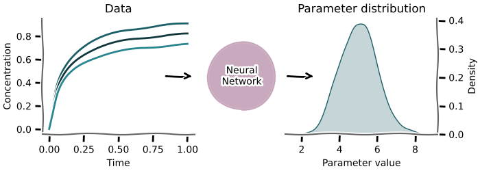
Neural posterior estimation¶

Neural posterior estimation answers the question: what parameters could have generated the data I measured?
Here you use an ODE model and prior knowledge about the parameters of interest to create synthetic data.
You then use the generated synthetic data as the features and the input parameters as the targets to train an inverse problem.
Once that training is successful, the neural network can now predict the input parameters for real world data.

You can use this technique for both steady-state as well as time course data.
The only difference is in using scan.time_course.

Take care here to save the targets as well in case you use cached data :)

In [2]:

# Note that now the parameters are the targets
npe_targets = sample(
    {
        "k1": LogNormal(mean=1.0, sigma=0.3),
    },
    n=1_000,
)

# And the generated data are the features
npe_features = (
    scan.steady_state(
        get_linear_chain_2v(),
        to_scan=npe_targets,
    )
    .get_args()
    .loc[:, ["y", "v2", "v3"]]
)

# It's always a good idea to check the inputs and outputs
fig, (ax1, ax2) = plot.two_axes(figsize=(6, 3), sharex=False)
_ = plot.violins(npe_features, ax=ax1)[1].set(title="Features", ylabel="Flux / a.u.")
_ = plot.violins(npe_targets, ax=ax2)[1].set(title="Targets", ylabel="Flux / a.u.")
plt.show()

# Note that now the parameters are the targets npe_targets = sample( { "k1": LogNormal(mean=1.0, sigma=0.3), }, n=1_000, ) # And the generated data are the features npe_features = ( scan.steady_state( get_linear_chain_2v(), to_scan=npe_targets, ) .get_args() .loc[:, ["y", "v2", "v3"]] ) # It's always a good idea to check the inputs and outputs fig, (ax1, ax2) = plot.two_axes(figsize=(6, 3), sharex=False) _ = plot.violins(npe_features, ax=ax1)[1].set(title="Features", ylabel="Flux / a.u.") _ = plot.violins(npe_targets, ax=ax2)[1].set(title="Targets", ylabel="Flux / a.u.") plt.show()

  0%|          | 0/1000 [00:00<?, ?it/s]

  0%|          | 1/1000 [00:05<1:28:02,  5.29s/it]

  0%|          | 2/1000 [00:05<37:30,  2.25s/it]  

  1%|          | 7/1000 [00:05<07:26,  2.22it/s]

  4%|▍         | 41/1000 [00:05<00:51, 18.67it/s]

  9%|▉         | 93/1000 [00:05<00:17, 51.26it/s]

 15%|█▍        | 147/1000 [00:05<00:09, 92.20it/s]

 20%|██        | 204/1000 [00:05<00:05, 142.15it/s]

 26%|██▌       | 259/1000 [00:06<00:03, 195.95it/s]

 31%|███       | 311/1000 [00:06<00:02, 247.04it/s]

 36%|███▌      | 362/1000 [00:06<00:02, 292.79it/s]

 42%|████▏     | 415/1000 [00:06<00:01, 341.59it/s]

 47%|████▋     | 468/1000 [00:06<00:01, 382.60it/s]

 52%|█████▏    | 520/1000 [00:06<00:01, 412.67it/s]

 57%|█████▋    | 572/1000 [00:06<00:00, 438.99it/s]

 62%|██████▏   | 623/1000 [00:06<00:01, 329.88it/s]

 67%|██████▋   | 674/1000 [00:07<00:00, 368.76it/s]

 73%|███████▎  | 726/1000 [00:07<00:00, 403.25it/s]

 78%|███████▊  | 776/1000 [00:07<00:00, 426.71it/s]

 83%|████████▎ | 829/1000 [00:07<00:00, 447.78it/s]

 88%|████████▊ | 879/1000 [00:07<00:00, 459.72it/s]

 93%|█████████▎| 934/1000 [00:07<00:00, 482.16it/s]

 98%|█████████▊| 985/1000 [00:07<00:00, 489.78it/s]

100%|██████████| 1000/1000 [00:07<00:00, 130.90it/s]

Train NPE¶

You can then train your neural posterior estimator using npe.train_torch_ss_estimator (or npe.train_torch_time_course_estimator if you have time course data).

In [3]:

estimator, losses = npe.torch.train_steady_state(
    features=npe_features,
    targets=npe_targets,
    epochs=100,
    batch_size=100,
)

ax = losses.plot(figsize=(4, 2.5))
ax.set(xlabel="epoch", ylabel="loss")
ax.set_ylim(0, None)
plt.show()

estimator, losses = npe.torch.train_steady_state( features=npe_features, targets=npe_targets, epochs=100, batch_size=100, ) ax = losses.plot(figsize=(4, 2.5)) ax.set(xlabel="epoch", ylabel="loss") ax.set_ylim(0, None) plt.show()

  0%|          | 0/100 [00:00<?, ?it/s]

 10%|█         | 10/100 [00:00<00:00, 96.18it/s]

 20%|██        | 20/100 [00:00<00:00, 95.73it/s]

 30%|███       | 30/100 [00:00<00:00, 96.81it/s]

 40%|████      | 40/100 [00:00<00:00, 97.28it/s]

 50%|█████     | 50/100 [00:00<00:00, 97.67it/s]

 60%|██████    | 60/100 [00:00<00:00, 97.92it/s]

 70%|███████   | 70/100 [00:00<00:00, 98.07it/s]

 80%|████████  | 80/100 [00:00<00:00, 98.26it/s]

 90%|█████████ | 90/100 [00:00<00:00, 98.18it/s]

100%|██████████| 100/100 [00:01<00:00, 98.27it/s]

100%|██████████| 100/100 [00:01<00:00, 97.75it/s]

Sanity check: do prior and posterior match?¶

In [4]:

fig, (ax1, ax2) = plot.two_axes(figsize=(6, 2))

ax = sns.kdeplot(npe_targets, fill=True, ax=ax1)
ax.set_title("Prior")

posterior = estimator.predict(npe_features)
ax = sns.kdeplot(posterior, fill=True, ax=ax2)
ax.set_title("Posterior")
plt.show()

fig, (ax1, ax2) = plot.two_axes(figsize=(6, 2)) ax = sns.kdeplot(npe_targets, fill=True, ax=ax1) ax.set_title("Prior") posterior = estimator.predict(npe_features) ax = sns.kdeplot(posterior, fill=True, ax=ax2) ax.set_title("Posterior") plt.show()

Re-entrant training¶

As with the surrogates you often you don't know the amount of epochs you are going to need in order to reach the required loss.
For the neural posterior estimation you can use the npe.TorchSteadyStateTrainer and npe.TorchTimeCourseTrainer respectively to continue training.

In [5]:

trainer = npe.torch.SteadyStateTrainer(
    features=npe_features,
    targets=npe_targets,
)

# Initial training
trainer.train(epochs=20, batch_size=100)
trainer.get_loss().plot(figsize=(4, 2.5)).set_ylim(0, None)
plt.show()

# Continue training
trainer.train(epochs=20, batch_size=100)
trainer.get_loss().plot(figsize=(4, 2.5)).set_ylim(0, None)
plt.show()

# Get trainer if loss is deemed suitable
estimator = trainer.get_estimator()

trainer = npe.torch.SteadyStateTrainer( features=npe_features, targets=npe_targets, ) # Initial training trainer.train(epochs=20, batch_size=100) trainer.get_loss().plot(figsize=(4, 2.5)).set_ylim(0, None) plt.show() # Continue training trainer.train(epochs=20, batch_size=100) trainer.get_loss().plot(figsize=(4, 2.5)).set_ylim(0, None) plt.show() # Get trainer if loss is deemed suitable estimator = trainer.get_estimator()

  0%|          | 0/20 [00:00<?, ?it/s]

 50%|█████     | 10/20 [00:00<00:00, 98.20it/s]

100%|██████████| 20/20 [00:00<00:00, 98.57it/s]

100%|██████████| 20/20 [00:00<00:00, 98.28it/s]

  0%|          | 0/20 [00:00<?, ?it/s]

 50%|█████     | 10/20 [00:00<00:00, 98.55it/s]

100%|██████████| 20/20 [00:00<00:00, 98.57it/s]

100%|██████████| 20/20 [00:00<00:00, 98.35it/s]

First finish line

With that you now know most of what you will need from a day-to-day basis about labelled models in mxlpy.

Congratulations!

Custom loss function¶

You can use a custom loss function by simply injecting a function that takes the predicted tensor x and the data y and produces another tensor.

In [6]:

from typing import TYPE_CHECKING

import torch

from mxlpy import LinearLabelMapper, Simulator
from mxlpy.distributions import sample
from mxlpy.fns import michaelis_menten_1s
from mxlpy.parallel import parallelise

if TYPE_CHECKING:
    from mxlpy import EstimatorProtocol

from typing import TYPE_CHECKING import torch from mxlpy import LinearLabelMapper, Simulator from mxlpy.distributions import sample from mxlpy.fns import michaelis_menten_1s from mxlpy.parallel import parallelise if TYPE_CHECKING: from mxlpy import EstimatorProtocol

In [7]:

def mean_abs(x: torch.Tensor, y: torch.Tensor) -> torch.Tensor:
    return torch.mean(torch.abs(x - y))


trainer = npe.torch.SteadyStateTrainer(
    features=npe_features,
    targets=npe_targets,
    loss_fn=mean_abs,
)

trainer = npe.torch.TimeCourseTrainer(
    features=npe_features,
    targets=npe_targets,
    loss_fn=mean_abs,
)

def mean_abs(x: torch.Tensor, y: torch.Tensor) -> torch.Tensor: return torch.mean(torch.abs(x - y)) trainer = npe.torch.SteadyStateTrainer( features=npe_features, targets=npe_targets, loss_fn=mean_abs, ) trainer = npe.torch.TimeCourseTrainer( features=npe_features, targets=npe_targets, loss_fn=mean_abs, )

Label NPE¶

In [8]:

# FIXME: todo
# Show how to change Adam settings or user other optimizers
# Show how to change the surrogate network

# FIXME: todo # Show how to change Adam settings or user other optimizers # Show how to change the surrogate network

In [9]:

def get_closed_cycle() -> tuple[Model, dict[str, int], dict[str, list[int]]]:
    """

    | Reaction       | Labelmap |
    | -------------- | -------- |
    | x1 ->[v1] x2   | [0, 1]   |
    | x2 ->[v2a] x3  | [0, 1]   |
    | x2 ->[v2b] x3  | [1, 0]   |
    | x3 ->[v3] x1   | [0, 1]   |

    """
    model = (
        Model()
        .add_parameters(
            {
                "vmax_1": 1.0,
                "km_1": 0.5,
                "vmax_2a": 1.0,
                "vmax_2b": 1.0,
                "km_2": 0.5,
                "vmax_3": 1.0,
                "km_3": 0.5,
            }
        )
        .add_variables({"x1": 1.0, "x2": 0.0, "x3": 0.0})
        .add_reaction(
            "v1",
            michaelis_menten_1s,
            stoichiometry={"x1": -1, "x2": 1},
            args=["x1", "vmax_1", "km_1"],
        )
        .add_reaction(
            "v2a",
            michaelis_menten_1s,
            stoichiometry={"x2": -1, "x3": 1},
            args=["x2", "vmax_2a", "km_2"],
        )
        .add_reaction(
            "v2b",
            michaelis_menten_1s,
            stoichiometry={"x2": -1, "x3": 1},
            args=["x2", "vmax_2b", "km_2"],
        )
        .add_reaction(
            "v3",
            michaelis_menten_1s,
            stoichiometry={"x3": -1, "x1": 1},
            args=["x3", "vmax_3", "km_3"],
        )
    )
    label_variables: dict[str, int] = {"x1": 2, "x2": 2, "x3": 2}
    label_maps: dict[str, list[int]] = {
        "v1": [0, 1],
        "v2a": [0, 1],
        "v2b": [1, 0],
        "v3": [0, 1],
    }
    return model, label_variables, label_maps

def get_closed_cycle() -> tuple[Model, dict[str, int], dict[str, list[int]]]: """ | Reaction | Labelmap | | -------------- | -------- | | x1 ->[v1] x2 | [0, 1] | | x2 ->[v2a] x3 | [0, 1] | | x2 ->[v2b] x3 | [1, 0] | | x3 ->[v3] x1 | [0, 1] | """ model = ( Model() .add_parameters( { "vmax_1": 1.0, "km_1": 0.5, "vmax_2a": 1.0, "vmax_2b": 1.0, "km_2": 0.5, "vmax_3": 1.0, "km_3": 0.5, } ) .add_variables({"x1": 1.0, "x2": 0.0, "x3": 0.0}) .add_reaction( "v1", michaelis_menten_1s, stoichiometry={"x1": -1, "x2": 1}, args=["x1", "vmax_1", "km_1"], ) .add_reaction( "v2a", michaelis_menten_1s, stoichiometry={"x2": -1, "x3": 1}, args=["x2", "vmax_2a", "km_2"], ) .add_reaction( "v2b", michaelis_menten_1s, stoichiometry={"x2": -1, "x3": 1}, args=["x2", "vmax_2b", "km_2"], ) .add_reaction( "v3", michaelis_menten_1s, stoichiometry={"x3": -1, "x1": 1}, args=["x3", "vmax_3", "km_3"], ) ) label_variables: dict[str, int] = {"x1": 2, "x2": 2, "x3": 2} label_maps: dict[str, list[int]] = { "v1": [0, 1], "v2a": [0, 1], "v2b": [1, 0], "v3": [0, 1], } return model, label_variables, label_maps

In [10]:

def _worker(
    x: tuple[tuple[int, pd.Series], tuple[int, pd.Series]],
    mapper: LinearLabelMapper,
    time: float,
    initial_labels: dict[str, int | list[int]],
) -> pd.Series:
    (_, y_ss), (_, v_ss) = x
    return (
        Simulator(mapper.build_model(y_ss, v_ss, initial_labels=initial_labels))
        .simulate(time)
        .get_result()
        .unwrap_or_err()
    ).variables.iloc[-1]


def get_label_distribution_at_time(
    model: Model,
    label_variables: dict[str, int],
    label_maps: dict[str, list[int]],
    time: float,
    initial_labels: dict[str, int | list[int]],
    ss_concs: pd.DataFrame,
    ss_fluxes: pd.DataFrame,
) -> pd.DataFrame:
    mapper = LinearLabelMapper(
        model,
        label_variables=label_variables,
        label_maps=label_maps,
    )

    return pd.DataFrame(
        dict(
            parallelise(
                partial(
                    _worker, mapper=mapper, time=time, initial_labels=initial_labels
                ),
                inputs=list(
                    enumerate(
                        zip(
                            ss_concs.iterrows(),
                            ss_fluxes.iterrows(),
                            strict=True,
                        )
                    )
                ),  # type: ignore
                cache=None,
            )
        ),
        dtype=float,
    ).T


def inverse_parameter_elasticity(
    estimator: EstimatorProtocol,
    datum: pd.Series,
    *,
    normalized: bool = True,
    displacement: float = 1e-4,
) -> pd.DataFrame:
    ref = estimator.predict(datum).iloc[0, :]

    coefs = {}
    for name, value in datum.items():
        up = coefs[name] = estimator.predict(
            pd.Series(datum.to_dict() | {name: value * 1 + displacement})
        ).iloc[0, :]
        down = coefs[name] = estimator.predict(
            pd.Series(datum.to_dict() | {name: value * 1 - displacement})
        ).iloc[0, :]
        coefs[name] = (up - down) / (2 * displacement * value)

    coefs = pd.DataFrame(coefs)
    if normalized:
        coefs *= datum / ref.to_numpy()

    return coefs

def _worker( x: tuple[tuple[int, pd.Series], tuple[int, pd.Series]], mapper: LinearLabelMapper, time: float, initial_labels: dict[str, int | list[int]], ) -> pd.Series: (_, y_ss), (_, v_ss) = x return ( Simulator(mapper.build_model(y_ss, v_ss, initial_labels=initial_labels)) .simulate(time) .get_result() .unwrap_or_err() ).variables.iloc[-1] def get_label_distribution_at_time( model: Model, label_variables: dict[str, int], label_maps: dict[str, list[int]], time: float, initial_labels: dict[str, int | list[int]], ss_concs: pd.DataFrame, ss_fluxes: pd.DataFrame, ) -> pd.DataFrame: mapper = LinearLabelMapper( model, label_variables=label_variables, label_maps=label_maps, ) return pd.DataFrame( dict( parallelise( partial( _worker, mapper=mapper, time=time, initial_labels=initial_labels ), inputs=list( enumerate( zip( ss_concs.iterrows(), ss_fluxes.iterrows(), strict=True, ) ) ), # type: ignore cache=None, ) ), dtype=float, ).T def inverse_parameter_elasticity( estimator: EstimatorProtocol, datum: pd.Series, *, normalized: bool = True, displacement: float = 1e-4, ) -> pd.DataFrame: ref = estimator.predict(datum).iloc[0, :] coefs = {} for name, value in datum.items(): up = coefs[name] = estimator.predict( pd.Series(datum.to_dict() | {name: value * 1 + displacement}) ).iloc[0, :] down = coefs[name] = estimator.predict( pd.Series(datum.to_dict() | {name: value * 1 - displacement}) ).iloc[0, :] coefs[name] = (up - down) / (2 * displacement * value) coefs = pd.DataFrame(coefs) if normalized: coefs *= datum / ref.to_numpy() return coefs

In [11]:

model, label_variables, label_maps = get_closed_cycle()

ss_concs, ss_fluxes = (
    Simulator(model)
    .update_parameters({"vmax_2a": 1.0, "vmax_2b": 0.5})
    .simulate_to_steady_state()
    .get_result()
    .unwrap_or_err()
)
mapper = LinearLabelMapper(
    model,
    label_variables=label_variables,
    label_maps=label_maps,
)

_, axs = plot.relative_label_distribution(
    mapper,
    (
        Simulator(
            mapper.build_model(
                ss_concs.iloc[-1], ss_fluxes.iloc[-1], initial_labels={"x1": 0}
            )
        )
        .simulate(5)
        .get_result()
        .unwrap_or_err()
    ).variables,
    sharey=True,
    n_cols=3,
)

axs[0, 0].set_ylabel("Relative label distribution")
axs[0, 1].set_xlabel("Time / s")
plt.show()

model, label_variables, label_maps = get_closed_cycle() ss_concs, ss_fluxes = ( Simulator(model) .update_parameters({"vmax_2a": 1.0, "vmax_2b": 0.5}) .simulate_to_steady_state() .get_result() .unwrap_or_err() ) mapper = LinearLabelMapper( model, label_variables=label_variables, label_maps=label_maps, ) _, axs = plot.relative_label_distribution( mapper, ( Simulator( mapper.build_model( ss_concs.iloc[-1], ss_fluxes.iloc[-1], initial_labels={"x1": 0} ) ) .simulate(5) .get_result() .unwrap_or_err() ).variables, sharey=True, n_cols=3, ) axs[0, 0].set_ylabel("Relative label distribution") axs[0, 1].set_xlabel("Time / s") plt.show()

In [12]:

surrogate_targets = sample(
    {
        "vmax_2b": Normal(0.5, 0.1),
    },
    n=1000,
).clip(lower=0)

ax = sns.kdeplot(surrogate_targets, fill=True)
ax.set_title("Prior")

surrogate_targets = sample( { "vmax_2b": Normal(0.5, 0.1), }, n=1000, ).clip(lower=0) ax = sns.kdeplot(surrogate_targets, fill=True) ax.set_title("Prior")

Out[12]:

Text(0.5, 1.0, 'Prior')

In [13]:

ss_concs, ss_fluxes = scan.steady_state(
    model,
    to_scan=surrogate_targets,
)

ss_concs, ss_fluxes = scan.steady_state( model, to_scan=surrogate_targets, )

  0%|          | 0/1000 [00:00<?, ?it/s]

  0%|          | 1/1000 [00:05<1:30:21,  5.43s/it]

  1%|          | 7/1000 [00:05<09:38,  1.72it/s]  

  2%|▏         | 23/1000 [00:05<02:13,  7.30it/s]

  6%|▌         | 60/1000 [00:05<00:38, 24.68it/s]

 10%|█         | 103/1000 [00:05<00:17, 50.65it/s]

 15%|█▍        | 146/1000 [00:05<00:10, 82.37it/s]

 19%|█▉        | 188/1000 [00:06<00:06, 117.98it/s]

 23%|██▎       | 230/1000 [00:06<00:05, 153.92it/s]

 27%|██▋       | 266/1000 [00:06<00:05, 134.04it/s]

 31%|███       | 307/1000 [00:06<00:04, 172.09it/s]

 35%|███▍      | 349/1000 [00:06<00:03, 210.69it/s]

 39%|███▉      | 391/1000 [00:06<00:02, 249.57it/s]

 43%|████▎     | 434/1000 [00:06<00:01, 285.39it/s]

 48%|████▊     | 476/1000 [00:07<00:01, 316.06it/s]

 52%|█████▏    | 516/1000 [00:07<00:01, 333.95it/s]

 56%|█████▌    | 558/1000 [00:07<00:01, 354.85it/s]

 60%|█████▉    | 598/1000 [00:07<00:01, 366.48it/s]

 64%|██████▍   | 640/1000 [00:07<00:00, 379.93it/s]

 68%|██████▊   | 682/1000 [00:07<00:00, 391.11it/s]

 72%|███████▏  | 723/1000 [00:07<00:00, 390.38it/s]

 76%|███████▋  | 765/1000 [00:07<00:00, 397.14it/s]

 81%|████████  | 809/1000 [00:07<00:00, 403.46it/s]

 85%|████████▌ | 852/1000 [00:07<00:00, 410.00it/s]

 89%|████████▉ | 894/1000 [00:08<00:00, 406.98it/s]

 94%|█████████▎| 937/1000 [00:08<00:00, 409.73it/s]

 98%|█████████▊| 979/1000 [00:08<00:00, 409.46it/s]

100%|██████████| 1000/1000 [00:08<00:00, 120.47it/s]

In [14]:

fig, (ax1, ax2) = plt.subplots(1, 2, figsize=(12, 4))
_, ax = plot.violins(ss_concs, ax=ax1)
ax.set_ylabel("Concentration / a.u.")
_, ax = plot.violins(ss_fluxes, ax=ax2)
ax.set_ylabel("Flux / a.u.")

fig, (ax1, ax2) = plt.subplots(1, 2, figsize=(12, 4)) _, ax = plot.violins(ss_concs, ax=ax1) ax.set_ylabel("Concentration / a.u.") _, ax = plot.violins(ss_fluxes, ax=ax2) ax.set_ylabel("Flux / a.u.")

Out[14]:

Text(0, 0.5, 'Flux / a.u.')

In [15]:

surrogate_features = get_label_distribution_at_time(
    model=model,
    label_variables=label_variables,
    label_maps=label_maps,
    time=5,
    ss_concs=ss_concs,
    ss_fluxes=ss_fluxes,
    initial_labels={"x1": 0},
)
_, ax = plot.violins(surrogate_features)
ax.set_ylabel("Relative label distribution")

surrogate_features = get_label_distribution_at_time( model=model, label_variables=label_variables, label_maps=label_maps, time=5, ss_concs=ss_concs, ss_fluxes=ss_fluxes, initial_labels={"x1": 0}, ) _, ax = plot.violins(surrogate_features) ax.set_ylabel("Relative label distribution")

  0%|          | 0/1000 [00:00<?, ?it/s]

  0%|          | 1/1000 [00:05<1:28:15,  5.30s/it]

  0%|          | 4/1000 [00:05<17:09,  1.03s/it]  

  1%|          | 6/1000 [00:05<10:05,  1.64it/s]

  2%|▏         | 18/1000 [00:05<02:13,  7.37it/s]

  4%|▍         | 38/1000 [00:05<00:48, 19.73it/s]

  6%|▌         | 56/1000 [00:05<00:28, 33.16it/s]

  8%|▊         | 76/1000 [00:05<00:18, 50.34it/s]

 10%|▉         | 96/1000 [00:06<00:12, 69.73it/s]

 12%|█▏        | 115/1000 [00:06<00:10, 88.47it/s]

 14%|█▎        | 135/1000 [00:06<00:08, 106.85it/s]

 16%|█▌        | 155/1000 [00:06<00:06, 123.77it/s]

 17%|█▋        | 174/1000 [00:06<00:06, 137.56it/s]

 19%|█▉        | 193/1000 [00:06<00:05, 148.17it/s]

 21%|██        | 212/1000 [00:06<00:04, 157.94it/s]

 23%|██▎       | 231/1000 [00:06<00:04, 163.28it/s]

 25%|██▍       | 249/1000 [00:06<00:04, 166.48it/s]

 27%|██▋       | 267/1000 [00:07<00:04, 169.40it/s]

 29%|██▊       | 286/1000 [00:07<00:04, 174.99it/s]

 30%|███       | 305/1000 [00:07<00:03, 177.15it/s]

 32%|███▏      | 324/1000 [00:07<00:03, 179.52it/s]

 34%|███▍      | 343/1000 [00:07<00:03, 181.02it/s]

 36%|███▋      | 365/1000 [00:07<00:03, 185.88it/s]

 39%|███▊      | 386/1000 [00:07<00:03, 190.65it/s]

 41%|████      | 406/1000 [00:07<00:03, 187.37it/s]

 42%|████▎     | 425/1000 [00:07<00:03, 186.41it/s]

 45%|████▍     | 446/1000 [00:07<00:02, 189.49it/s]

 46%|████▋     | 465/1000 [00:08<00:02, 186.57it/s]

 48%|████▊     | 485/1000 [00:08<00:02, 189.20it/s]

 50%|█████     | 504/1000 [00:08<00:02, 188.49it/s]

 52%|█████▏    | 523/1000 [00:08<00:02, 186.07it/s]

 54%|█████▍    | 542/1000 [00:08<00:02, 182.52it/s]

 56%|█████▌    | 561/1000 [00:08<00:02, 183.21it/s]

 58%|█████▊    | 580/1000 [00:08<00:02, 180.36it/s]

 60%|█████▉    | 599/1000 [00:08<00:02, 180.07it/s]

 62%|██████▏   | 618/1000 [00:08<00:02, 179.68it/s]

 64%|██████▎   | 637/1000 [00:09<00:02, 180.52it/s]

 66%|██████▌   | 656/1000 [00:09<00:01, 181.74it/s]

 68%|██████▊   | 675/1000 [00:09<00:01, 181.93it/s]

 69%|██████▉   | 694/1000 [00:09<00:01, 184.26it/s]

 71%|███████▏  | 713/1000 [00:09<00:01, 181.68it/s]

 74%|███████▎  | 735/1000 [00:09<00:01, 187.37it/s]

 75%|███████▌  | 754/1000 [00:09<00:01, 186.89it/s]

 77%|███████▋  | 773/1000 [00:09<00:01, 185.89it/s]

 79%|███████▉  | 794/1000 [00:09<00:01, 188.54it/s]

 81%|████████▏ | 813/1000 [00:09<00:00, 188.01it/s]

 83%|████████▎ | 832/1000 [00:10<00:00, 187.90it/s]

 85%|████████▌ | 851/1000 [00:10<00:00, 185.74it/s]

 87%|████████▋ | 870/1000 [00:10<00:00, 184.43it/s]

 89%|████████▉ | 890/1000 [00:10<00:00, 184.45it/s]

 91%|█████████ | 911/1000 [00:10<00:00, 186.17it/s]

 93%|█████████▎| 930/1000 [00:10<00:00, 186.23it/s]

 95%|█████████▍| 949/1000 [00:10<00:00, 186.22it/s]

 97%|█████████▋| 968/1000 [00:10<00:00, 185.91it/s]

 99%|█████████▊| 987/1000 [00:10<00:00, 186.03it/s]

100%|██████████| 1000/1000 [00:10<00:00, 91.36it/s]

Out[15]:

Text(0, 0.5, 'Relative label distribution')

In [16]:

estimator, losses = npe.torch.train_steady_state(
    features=surrogate_features,
    targets=surrogate_targets,
    batch_size=100,
    epochs=250,
)

ax = losses.plot()
ax.set_ylim(0, None)

estimator, losses = npe.torch.train_steady_state( features=surrogate_features, targets=surrogate_targets, batch_size=100, epochs=250, ) ax = losses.plot() ax.set_ylim(0, None)

  0%|          | 0/250 [00:00<?, ?it/s]

  3%|▎         | 8/250 [00:00<00:03, 72.91it/s]

  7%|▋         | 18/250 [00:00<00:02, 88.07it/s]

 11%|█         | 28/250 [00:00<00:02, 93.29it/s]

 15%|█▌        | 38/250 [00:00<00:02, 95.84it/s]

 20%|█▉        | 49/250 [00:00<00:02, 97.40it/s]

 24%|██▎       | 59/250 [00:00<00:01, 98.22it/s]

 28%|██▊       | 69/250 [00:00<00:01, 98.45it/s]

 32%|███▏      | 79/250 [00:00<00:01, 98.66it/s]

 36%|███▌      | 89/250 [00:00<00:01, 98.77it/s]

 40%|███▉      | 99/250 [00:01<00:01, 99.11it/s]

 44%|████▎     | 109/250 [00:01<00:01, 99.25it/s]

 48%|████▊     | 120/250 [00:01<00:01, 99.59it/s]

 52%|█████▏    | 131/250 [00:01<00:01, 99.81it/s]

 56%|█████▋    | 141/250 [00:01<00:01, 99.81it/s]

 60%|██████    | 151/250 [00:01<00:00, 99.79it/s]

 64%|██████▍   | 161/250 [00:01<00:00, 99.69it/s]

 68%|██████▊   | 171/250 [00:01<00:00, 99.52it/s]

 72%|███████▏  | 181/250 [00:01<00:00, 99.32it/s]

 76%|███████▋  | 191/250 [00:01<00:00, 99.48it/s]

 80%|████████  | 201/250 [00:02<00:00, 99.43it/s]

 84%|████████▍ | 211/250 [00:02<00:00, 97.93it/s]

 88%|████████▊ | 221/250 [00:02<00:00, 98.00it/s]

 92%|█████████▏| 231/250 [00:02<00:00, 97.05it/s]

 96%|█████████▋| 241/250 [00:02<00:00, 96.87it/s]

100%|██████████| 250/250 [00:02<00:00, 97.58it/s]

Out[16]:

(0.0, 0.5100764895405154)

In [17]:

fig, (ax1, ax2) = plt.subplots(
    1,
    2,
    figsize=(8, 3),
    layout="constrained",
    sharex=True,
    sharey=False,
)

ax = sns.kdeplot(surrogate_targets, fill=True, ax=ax1)
ax.set_title("Prior")

posterior = estimator.predict(surrogate_features)

ax = sns.kdeplot(posterior, fill=True, ax=ax2)
ax.set_title("Posterior")
ax2.set_ylim(*ax1.get_ylim())
plt.show()

fig, (ax1, ax2) = plt.subplots( 1, 2, figsize=(8, 3), layout="constrained", sharex=True, sharey=False, ) ax = sns.kdeplot(surrogate_targets, fill=True, ax=ax1) ax.set_title("Prior") posterior = estimator.predict(surrogate_features) ax = sns.kdeplot(posterior, fill=True, ax=ax2) ax.set_title("Posterior") ax2.set_ylim(*ax1.get_ylim()) plt.show()

Inverse parameter sensitivity¶

In [18]:

_ = plot.heatmap(inverse_parameter_elasticity(estimator, surrogate_features.iloc[0]))

_ = plot.heatmap(inverse_parameter_elasticity(estimator, surrogate_features.iloc[0]))

In [19]:

elasticities = pd.DataFrame(
    {
        k: inverse_parameter_elasticity(estimator, i).loc["vmax_2b"]
        for k, i in surrogate_features.iterrows()
    }
).T

_ = plot.violins(elasticities)

elasticities = pd.DataFrame( { k: inverse_parameter_elasticity(estimator, i).loc["vmax_2b"] for k, i in surrogate_features.iterrows() } ).T _ = plot.violins(elasticities)

In [ ]: